Custom tree visualization

This page demonstrates custom tree visualization options available in the Python API, including custom colormaps, and may be used for developing visualizations in a Jupyter notebook. See docs page on the CollapsedTree.render() method for more details.

Import packages

import gctree
import pickle
import numpy as np

Load an inferred CollapsedTree object from a pickle file (such as are output by the gctree CLI)

with open("gctree.out.inference.1.p", "rb") as f:
    tree = pickle.load(f)

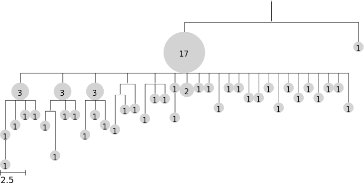
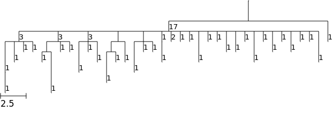
The default tree rendering

Note that the special file name "%%inline" allows rendering in the notebook. To render to a file, supply a filename instead, e.g. "tree1.svg"

tree.render("%%inline")

Rendering arguments

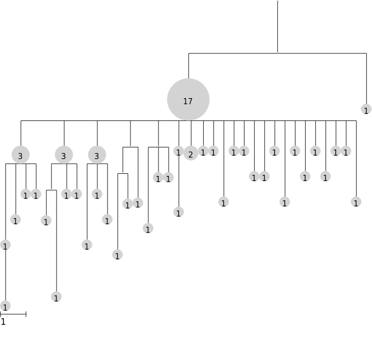
Use the scale argument to make the tree taller

tree.render("%%inline", scale=50)

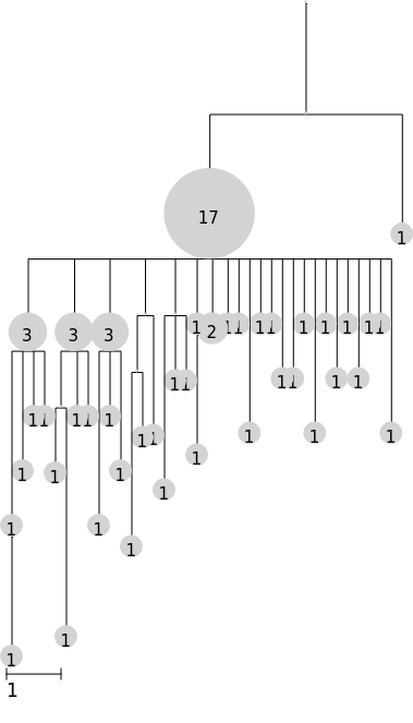
Use the branch_margin argument to compress (negative) or expand (positive) tree width

tree.render("%%inline", scale=50, branch_margin=-10)

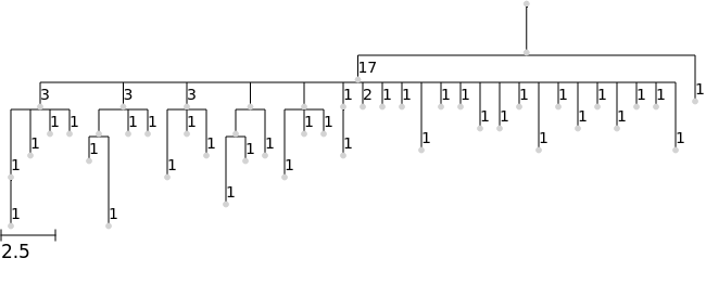
Instead of the default node sizing by abundance, set a fixed size with the node_size argument

tree.render("%%inline", node_size=5)

To make nodes disappear (e.g. for consistent root-to-tip heights) you can set node_size=0

tree.render("%%inline", node_size=0)

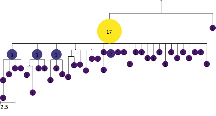
Coloring nodes

The argument colormap can be used to customize the colors of nodes. You can supply a dictionary with node names as keys and with values that are color names in ETE or RGB hex values.

Here we will instead demonstrate how to use a custom colormap based on a numerical node feature. We will use node abundance feature (which all gctree trees have) in this example, and will use the "viridis" palette for our color range. You can use other named palettes shown here.

We first obtain the color map based on the abundance feature, and then supply this as the colormap argument when rendering. See docs page on the CollapsedTree.feature_colormap() method for more details.

colormap = tree.feature_colormap("abundance")
tree.render("%%inline", colormap=colormap)

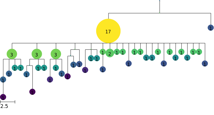
Local branching statistics

We might want to color by other node attributes, and here we show how to compute the local branching index (LBI) (Neher et al., 2014) to measure “bushiness”, which may be associated with fitness.

• The method local_branching() computes LBI for all nodes in our tree, and assigns them as tree features. See docs page on the CollapsedTree.local_branching() method for more details.

• We then create a colormap based on these features, using the scale argument to specify log scale.

• Finally, we use this colormap to render a tree with nodes colored by LBI

tree.local_branching()
colormap = tree.feature_colormap("LBI", scale="log")
tree.render("%%inline", colormap=colormap)

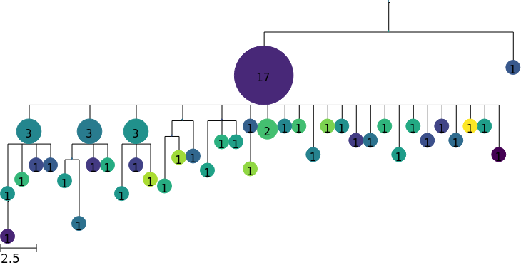
Custom node features

We can use any numerical node feature to color our tree. For example, we might have affinity estimates for each node.

In this example, we assign random values as node features to create artificial affinity data. With real data, we would assign values based on the node.name or node.sequence of each node.

for node in tree.tree.traverse():
    node.add_feature("affinity", np.random.randn())

colormap = tree.feature_colormap("affinity")
tree.render("%%inline", colormap=colormap)