Simulation validation
Overview
The bloom lab had developed a pipeline to simulate DMS data to test dms_variants global epistasis fitting. Taking inspriation from that, we build upon the pipeline by simulating data for two homologs - introducing shifts in mutational effects at a subset of sites with the goal validating the multidms joint-fitting approach.
This notebook has a few major steps involved:
Simulate sequences, and respective mutational effects for two homologs – introducing shifts at a subset of sites for the non-reference homolog.
Define replicate libraries of variants for each homolog.
Simulating pre, and post-selection library variant counts derived from a simulated bottleneck and used to introduce realistic noise in the fitting targets (functional scores).
multidmsmodel fitting.Model fit comparison and selection criteria
Model evaluation.
Import Python modules
For this analysis, we’ll be using the dms_variants package for simulation. All dependencies needed can be installed by cloning the multidms repo and executing the command:
$ pip install '.[dev]'
[1]:
import warnings
import pprint
import os

import pandas as pd
import numpy as np
import matplotlib.pyplot as plt
import seaborn as sns

import Bio.Seq
import itertools
import random
import dms_variants.codonvarianttable
import dms_variants.globalepistasis
import dms_variants.plotnine_themes
import dms_variants.simulate
from dms_variants.constants import CBPALETTE, CODONS_NOSTOP, AAS_NOSTOP, AA_TO_CODONS, AAS_WITHSTOP
from plotnine import *
import multidms
from collections import defaultdict
Define notebook parameters
Set parameters that define this notebook’s behavior. These can all be modifed (using papermill) to reasonable values and the notebook should execute as expected.
[2]:
seed = 24  # random number seed

# define the reference protein sequence we're going to simulate
genelength = 50  # gene length in codons
wt_latent = 5.0 # wildtype latent phenotype
stop_effect = -15 # -15 is the default for `SigmoidPhenotypeSimulator` object
norm_weights=((0.4, -0.5, 1.2), (0.6, -4, 3)) # See `SigmoidPhenotypeSimulator` for more details

# define the non reference sequence attributes.
n_non_identical_sites = 10 # number of amino-acid mutations separating homologs
min_muteffect_in_bundle = -1.0 # minimum effect per mutation
max_muteffect_in_bundle = 1.0 # maximum effect per mutation
n_shifted_non_identical_sites = 6 # number of non identical sites (in the bundle) for which mutations at that site are expected to have shifted effects
n_shifted_identical_sites = 4 # number of amino-acid mutations separating shifted
shift_gauss_variance = 1.0 # variance of the gaussian distribution from which the shifted effects are drawn

# define the sigmoid phenotype parameters. See `multidms.biophysical.sigmoidal_global_epistasis` for more details.
sigmoid_phenotype_scale = 6

# define the libraries
variants_per_lib_genelength_scalar = 500  # variants per library
avgmuts = 2.0  # average codon mutations per variant
bclen = 16  # length of nucleotide barcode for each variant
variant_error_rate = 0.0 #0.005  # rate at which variant sequence mis-called
avgdepth_per_variant = 200  # average per-variant sequencing depth
lib_uniformity = 5  # uniformity of library pre-selection
noise = 0.0 # 0.05 # random gaussian noise added to the post-selection counts of the phenotype

# bottlenecks from pre- to post-selection
bottleneck_variants_per_lib_scalar = {
    "tight_bottle": 5,
    "loose_bottle": 100,
}

# define the fitting parameters
maxiter = 100000 # default 20000
tol=1e-3
scale_coeff_lasso_shift = [0.0, 5.00e-6, 1.00e-05, 2.00e-05, 4.00e-05, 8.00e-05, 1.60e-04, 3.20e-04, 6.40e-04] # the sweep of lasso coefficient params
init_beta_naught = 5.0 # We've found that we need to start with a higher beta_naught to get the model to converge correctly,
scale_coeff_ridge_beta = 1e-7 # the sweep of ridge coefficient params
train_frac = 0.8 # fraction of data to use for cross validation training.
lasso_choice = 8e-5 # the lasso coefficient to use for the final model
csv_output_dir = 'output' # the directory to save the output csv files
Set some configurations and a few other more experimental parameters which could break things if not set correctly:
[3]:
%matplotlib inline

random.seed(seed)
np.random.seed(seed)
warnings.simplefilter('ignore')

if not os.path.exists(csv_output_dir):
    os.makedirs(csv_output_dir)
Simulate a reference sequence
Start by simulating a sequence of nucleotides, then translate it to amino acids. We’ll use this sequence as the reference sequence for the simulated datasets.
[4]:
geneseq_h1 = "".join(random.choices(CODONS_NOSTOP, k=genelength))
aaseq_h1 = str(Bio.Seq.Seq(geneseq_h1).translate())
print(f"Wildtype gene of {genelength} codons:\n{geneseq_h1}")
print(f"Wildtype protein:\n{aaseq_h1}")
Wildtype gene of 50 codons:
GGTTCCAGTTTTAGTGGAACCGTGAGCGGTGTAGTGCGGTCGTTTACTCTTTTCGTCCGTCAGTTCACCGTGTCCAGCCATCAGGACCCGTGCTGTCATTGCACAACCGGATACTATTTTTCGCAAGTCTGTACCCTGAGCAGACTCGGA
Wildtype protein:
GSSFSGTVSGVVRSFTLFVRQFTVSSHQDPCCHCTTGYYFSQVCTLSRLG
Mutational effects
Simulate latent mutational effects, \(\beta_m\), storing data in a SigmoidPhenotypeSimulator object. Also create an identical object for the second homolog. Later, we’ll update this object to include shifted mutational effects.
[5]:
mut_pheno_args = {
    "geneseq" : geneseq_h1,
    "wt_latent" : wt_latent,
    "seed" : seed,
    "stop_effect" : stop_effect,
    "norm_weights" : norm_weights
}

SigmoidPhenotype_h1 = dms_variants.simulate.SigmoidPhenotypeSimulator(**mut_pheno_args)
SigmoidPhenotype_h2 = dms_variants.simulate.SigmoidPhenotypeSimulator(**mut_pheno_args)
Plot the distribution of mutation effects for the first homolog.
[6]:
p = (
    ggplot(pd.DataFrame({'muteffects': SigmoidPhenotype_h1.muteffects}),
           aes(x='muteffects'))
    + geom_histogram(binwidth=0.5, color='black', fill='pink', alpha=0.7)
    + xlab("mutation effect, $β$")
    + ylab('number of mutations')
    + theme_classic()
    + theme(figure_size=(5, 3))
)
_ = p.draw(show=True)
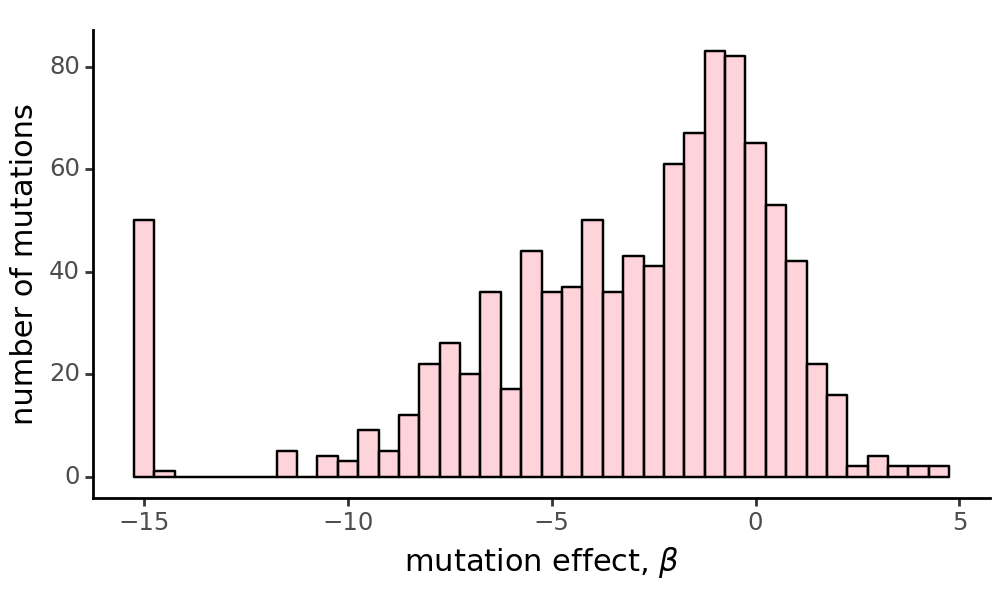
As expected, our mutational effects are weighted in the negative direction, as we expect the majority of mutations to be deleterious to a protein.
Non-reference homolog sequence
Next, we’ll simulate the DNA/protein sequence of second homolog by making a defined number of random amino-acid mutations to the first homolog. When choosing the “bundle” of mutation which separate the two homologs, we avoid mutations that decrease or increase the latent phenotype by more than min_muteffect_in_bundle and max_muteffect_in_bundle respectively. This is to ensure that the latent phenotype of the second homolog is not too different from the first homolog, an important
assumption for the multidms model.
[7]:
# Input params
non_identical_sites = sorted(random.sample(range(1, len(aaseq_h1)+1), n_non_identical_sites))
aaseq_h2 = ''
geneseq_h2 = ''


# Iterate over each amino acid in the first homolog, and make a mutation if indicated.
for (aa_n, aa) in enumerate(aaseq_h1, 1):
    codon = geneseq_h1[(aa_n-1)*3:3*aa_n]
    if aa_n in non_identical_sites:
        # define the valid mutations for this site
        valid_bundle_mutations = [
            mut_aa for mut_aa in AAS_NOSTOP
            if (
                (mut_aa != aa) \
                and (SigmoidPhenotype_h1.muteffects[f'{aa}{aa_n}{mut_aa}'] > min_muteffect_in_bundle) \
                and (SigmoidPhenotype_h1.muteffects[f'{aa}{aa_n}{mut_aa}'] < max_muteffect_in_bundle)
            )
        ]
        assert len(valid_bundle_mutations) > 0, aa_n
        mut_aa = random.choice(valid_bundle_mutations)
        aaseq_h2 += mut_aa
        mut_codon = random.choice(AA_TO_CODONS[mut_aa])
        geneseq_h2 += mut_codon
    else:
        aaseq_h2 += aa
        geneseq_h2 += codon

# Store and summarize results
homolog_seqs_df = pd.DataFrame(
    {"wt_aa_h1" : list(aaseq_h1), "wt_aa_h2" : list(aaseq_h2)},
    index = range(1, len(aaseq_h1)+1),
)
homolog_seqs_df.index.name = 'site'

# n_diffs = sum([aa1 != aa2 for (aa1, aa2) in zip(*homolog_seqs.values())])
n_diffs = len(homolog_seqs_df.query('wt_aa_h1 != wt_aa_h2'))
print('Sequence alignment of homologs h1 and h2:')
print('h1', aaseq_h1)
print('h2', aaseq_h2)
print('Number of aa differences:', n_diffs)
assert len(aaseq_h1) == len(aaseq_h2)
assert aaseq_h2 == str(Bio.Seq.Seq(geneseq_h2).translate())
assert n_diffs == len(non_identical_sites)
Sequence alignment of homologs h1 and h2:
h1 GSSFSGTVSGVVRSFTLFVRQFTVSSHQDPCCHCTTGYYFSQVCTLSRLG
h2 GSSFSGTGEGVVRMFTLFVRQFTVSSHQDPCDHCITSDYFSHVETLSRVG
Number of aa differences: 10
Shifted mutational effects
Next, randomly choose a subset of (identical and non-identical) sites that will have shifted mutational effects. Do this independently for sites that are identical and non-identical between homologs, so that we are sure to have shifted sites in each category.
[8]:
# Non-identical sites
shifted_non_identical_sites = sorted(random.sample(
    non_identical_sites,
    n_shifted_non_identical_sites
))

# choose a subset of the identical sites to have shifted effects
shifted_identical_sites = sorted(random.sample(
    list(set(range(1, len(aaseq_h1)+1)) - set(non_identical_sites)),
    n_shifted_identical_sites
))

# Make a list of all shifted sites
shifted_sites = sorted(shifted_identical_sites + shifted_non_identical_sites)
assert len(shifted_sites) == len(set(shifted_sites))
print('Sites with shifts that are...')
print(f'identical (n={len(shifted_identical_sites)}):', ', '.join(map(str, shifted_identical_sites)))
print(f'non-identical (n={len(shifted_non_identical_sites)}):', ', '.join(map(str, shifted_non_identical_sites)))
Sites with shifts that are...
identical (n=4): 30, 34, 39, 48
non-identical (n=6): 8, 14, 32, 37, 38, 42
Next, we’ll create a dataframe for all mutational effects and shifts, simulating shifts at each of the above sites by randomly simulate a shift in the effect of each mutation by drawing shifts from a Gaussian distribution:
[9]:
def sim_mut_shift(shifted_site, mutation):
    if (not shifted_site) or ('*' in mutation):
        return 0
    else:
        return np.random.normal(loc=0, scale=shift_gauss_variance, size=1)[0]

# Make a dataframe of mutation effects in the first homolog
mut_effects_df = (
    pd.DataFrame.from_dict(
        SigmoidPhenotype_h1.muteffects,
        orient='index',
        columns=['beta_h1']
    )
    .reset_index()
    .rename(columns={'index':'mutation'})
    .assign(
        wt_aa=lambda x: x['mutation'].apply(lambda y: multidms.data.split_sub(y)[0]),
        site=lambda x: x['mutation'].apply(lambda y: int(multidms.data.split_sub(y)[1])),
        mut_aa=lambda x: x['mutation'].apply(lambda y: multidms.data.split_sub(y)[2]),
        shifted_site=lambda x: x['site'].isin(shifted_sites),
        shift=lambda x: x.apply(
            lambda row: sim_mut_shift(
                row['shifted_site'],
                row['mutation']
            ),
            axis=1
        ),
        beta_h2=lambda x: x['beta_h1'] + x['shift']
    )
    .merge(homolog_seqs_df, left_on='site', right_index=True, how='left')
    .assign(
        bundle_mut = lambda x: x['mut_aa'] == x['wt_aa_h2']
    )
)

# Show data for a subset of sites with shifts
mut_effects_df[mut_effects_df['shifted_site'] == True][[
    'site', 'wt_aa_h1', 'wt_aa_h2', 'mutation',
    'beta_h1', 'shift', 'beta_h2',
    'shifted_site'
]]
[9]:
| site | wt_aa_h1 | wt_aa_h2 | mutation | beta_h1 | shift | beta_h2 | shifted_site | |
|---|---|---|---|---|---|---|---|---|
| 140 | 8 | V | G | V8A | -7.389801 | 1.329212 | -6.060588 | True |
| 141 | 8 | V | G | V8C | -7.620390 | -0.770033 | -8.390423 | True |
| 142 | 8 | V | G | V8D | -7.295378 | -0.316280 | -7.611658 | True |
| 143 | 8 | V | G | V8E | -0.729143 | -0.990810 | -1.719953 | True |
| 144 | 8 | V | G | V8F | -1.369987 | -1.070816 | -2.440803 | True |
| ... | ... | ... | ... | ... | ... | ... | ... | ... |
| 955 | 48 | R | R | R48T | -6.008805 | -2.870096 | -8.878901 | True |
| 956 | 48 | R | R | R48V | 0.899548 | 0.351710 | 1.251258 | True |
| 957 | 48 | R | R | R48W | -8.789600 | 0.265490 | -8.524110 | True |
| 958 | 48 | R | R | R48Y | -5.326602 | 0.105712 | -5.220890 | True |
| 959 | 48 | R | R | R48* | -15.000000 | 0.000000 | -15.000000 | True |
200 rows × 8 columns
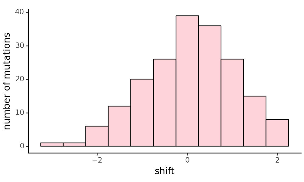
Plot the distribution of all simulated shifts, excluding mutations to stop codons and sites that have no shifted effects.
[10]:
non_stop_shifted_muts = mut_effects_df[
    (mut_effects_df['site'].isin(shifted_sites)) &
    ~(mut_effects_df['mutation'].str.contains('\*'))
]

p = (
    ggplot(non_stop_shifted_muts, aes(x='shift'))
    + geom_histogram(binwidth=0.5, color='black', fill='pink', alpha=0.7)
    + xlab("shift")
    + ylab('number of mutations')
    + theme_classic()
    + theme(figure_size=(5, 3))
)

_ = p.draw(show=True)
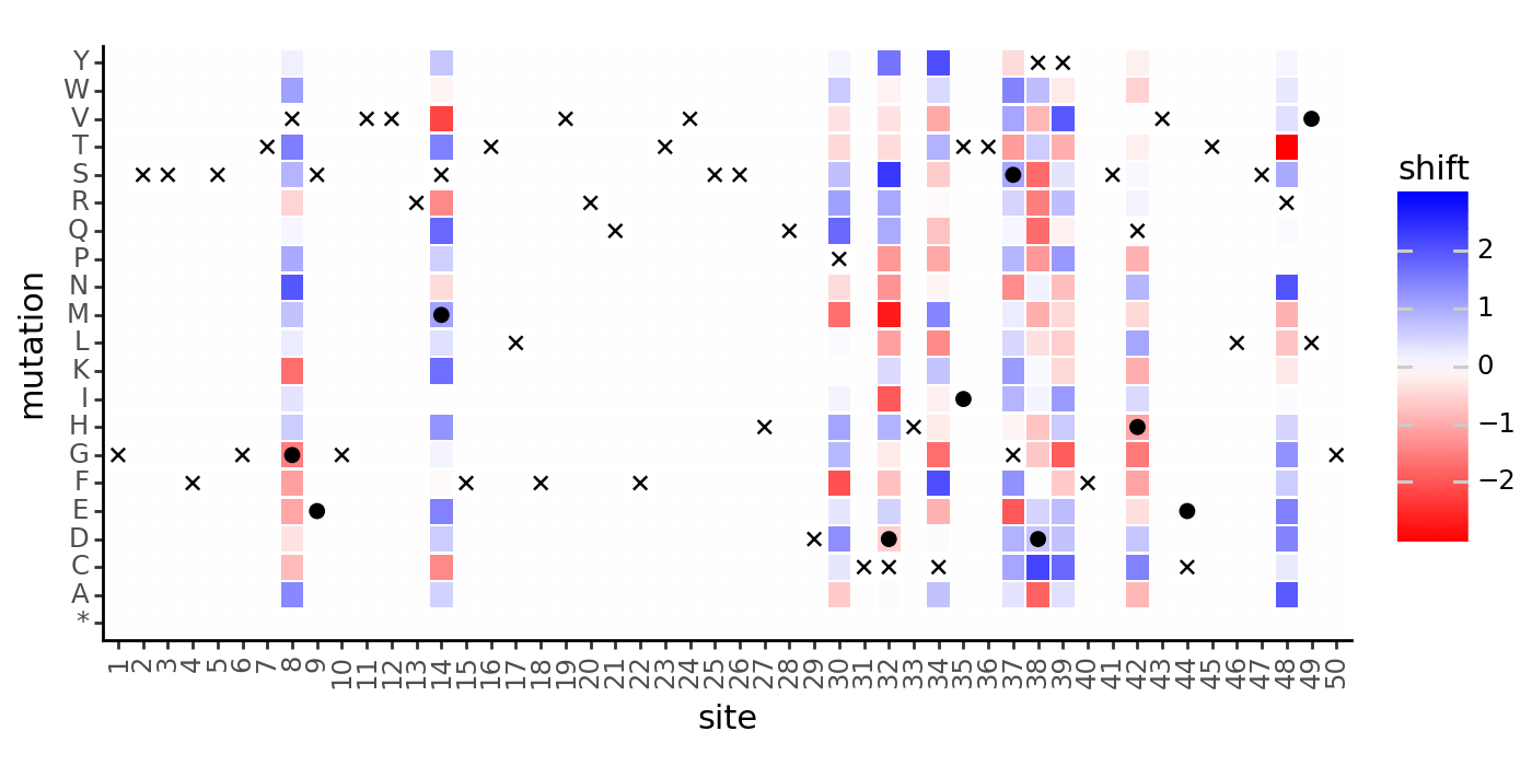
We can also plot the shifts as a heatmap, and mark the wildtype amino acid at each site (x for reference, o for non-reference):
[11]:
max_abs_value = max(abs(mut_effects_df['shift'].min()), mut_effects_df['shift'].max())
x_scale = [s for s in range(1, len(homolog_seqs_df)+1)]
y_scale = sorted([
    "R","K","H","D","E","Q","N","S",
    "T","Y","W","F","A","I","L","M",
    "V","G","P","C","*",
])

p = (
    ggplot(mut_effects_df)
    + geom_tile(
        aes(x='factor(site)', y='mut_aa', fill='shift', width=.9, height=.9)
    )
    + geom_point(
        homolog_seqs_df.reset_index(),
        aes(
            x='factor(site)', y='wt_aa_h1' #, label='aaseq_h1'
        ),
        color='black',
        size=2,
        shape='x'
    )
    + geom_point(
        homolog_seqs_df.reset_index().query('wt_aa_h1 != wt_aa_h2'),
        aes(
            x='factor(site)', y='wt_aa_h2'
        ),
        color='black',
        size=2,
        shape='o'
    )
    + scale_x_discrete(
        limits = x_scale,
        labels = x_scale
    )
    + scale_y_discrete(
        limits = y_scale,
        labels = y_scale
    )
    + scale_fill_gradientn(
        colors=['red', 'white', 'blue'],
        limits=[-max_abs_value, max_abs_value],
    )
    + theme_classic()
    + theme(
        axis_text_x=element_text(angle=90),
        figure_size=(7, 3.5)
    )
    + xlab('site')
    + ylab('mutation')
)
_ = p.draw(show=True)
Recal that we have already created a SigmoidPhenotypeSimulator object for the second homolog by making a copy of the one for the first homolog. This object stores the homolog’s wildtype latent phenotype and the latent effects of individual mutations. Below, we update both of these traits based on the simulated shifts from above. To update the wildtype latent phenotype of the second homolog, we add the effects of all mutations that separate the homologs. In computing this sum, we will use
\(\beta\) parameters for the second homolog, which already include shifted effects.
[12]:
# Update individual mutational effects
assert sum(mut_effects_df['mutation'].duplicated()) == 0
for mutation in SigmoidPhenotype_h2.muteffects.keys():
    SigmoidPhenotype_h2.muteffects[mutation] = mut_effects_df.loc[
        mut_effects_df['mutation']==mutation, 'beta_h2'
    ].values[0]

wt_latent_phenotype_shift = mut_effects_df.query("bundle_mut")["beta_h2"].sum()
SigmoidPhenotype_h2.wt_latent = SigmoidPhenotype_h1.wt_latent + wt_latent_phenotype_shift

print('Characteristics of mutations separating homologs:\n')
for metric in ['beta_h1', 'shift', 'beta_h2']:
    print(f'  Sum of {metric}:', round(sum(mut_effects_df.query("bundle_mut")[metric]), 2))
print('  Final WT latent phenotype of h2:', round(SigmoidPhenotype_h2.wt_latent, 2))
print('  Table of mutations that separate homologs:')
mut_effects_df.query("mut_aa == wt_aa_h2")
Characteristics of mutations separating homologs:

  Sum of beta_h1: 0.66
  Sum of shift: -0.28
  Sum of beta_h2: 0.38
  Final WT latent phenotype of h2: 5.38
  Table of mutations that separate homologs:
[12]:
| mutation | beta_h1 | wt_aa | site | mut_aa | shifted_site | shift | beta_h2 | wt_aa_h1 | wt_aa_h2 | bundle_mut | |
|---|---|---|---|---|---|---|---|---|---|---|---|
| 145 | V8G | 0.834349 | V | 8 | G | True | -1.438713 | -0.604364 | V | G | True |
| 163 | S9E | -0.705146 | S | 9 | E | False | 0.000000 | -0.705146 | S | E | True |
| 270 | S14M | 0.192719 | S | 14 | M | True | 1.037528 | 1.230247 | S | M | True |
| 621 | C32D | 0.958833 | C | 32 | D | True | -0.538963 | 0.419870 | C | D | True |
| 687 | T35I | 0.097535 | T | 35 | I | False | 0.000000 | 0.097535 | T | I | True |
| 734 | G37S | -0.695803 | G | 37 | S | True | 0.990621 | 0.294818 | G | S | True |
| 742 | Y38D | -0.265583 | Y | 38 | D | True | 0.669489 | 0.403906 | Y | D | True |
| 826 | Q42H | -0.888294 | Q | 42 | H | True | -0.996761 | -1.885055 | Q | H | True |
| 862 | C44E | 0.136021 | C | 44 | E | False | 0.000000 | 0.136021 | C | E | True |
| 976 | L49V | 0.996403 | L | 49 | V | False | 0.000000 | 0.996403 | L | V | True |
At this point, all mutations in the second homolog’s SigmoidPhenotypeSimulator object are defined relative to the wildtype sequence of the first homolog, which we will call the “reference” homolog. However, to compute phenotypes for the second homolog, we still need to assign the effects of mutations at non-identical sites in the “non-reference” homolog. For instance, if the wildtype amino acid at site 30 is an A in the reference homolog, but is a Y in a non-reference homolog, then the
effect of a Y30G is absent from the second homolog’s simulator object.
To add these missing entries, we will use a strategy that assumes additivity between mutations at the same site. For instance, in the above example, the effect of a Y30G mutation is defined as the sum of the A30Y (negated) and A30G effects in the reference homolog. This approach assumes that mutational effects can be negated, such that A30Y has the opposite effect as Y30A. It also assumes that mutational effects are additive, such that the effect of Y30G is the sum of the effects of Y30A and A30G.
The below expression defines this approach more explicitly for an arbitrary site. It uses the notation \(\beta_{x,n,z}\) where \(x\) and \(z\) are amino acids. For a site \(n\), if \(aa_{\text{wt}}\) is the site’s wildtype amino acid in a non-reference homolog, \(aa_{\text{mut}}\) is a mutant amino acid in a variant of that homolog, and \(aa_{\text{ref}}\) is the site’s wildtype amino acid in the reference homolog, then the mutation’s effect is:
The above \(\beta\) parameters are effects in the background of the non-reference homolog, such that they account for shifts in mutational effects between homologs.
The below cell adds mutational effects for missing entries using the above strategy:
[13]:
# iterate over "bundle" of mutations which disguish the homologs
for idx, row in mut_effects_df.query("mut_aa == wt_aa_h2").iterrows():

    # compute the effect of each possible mutation at a bundle site
    for aa_mut in AAS_WITHSTOP:

        # skip the non-ref wt-to-wt
        if aa_mut == row.wt_aa_h2:
            continue

        non_ref_mutation = f'{row.wt_aa_h2}{row.site}{aa_mut}'

        # stop effect is the same for all homologs
        if aa_mut == '*':
            SigmoidPhenotype_h2.muteffects[non_ref_mutation] = stop_effect

        # back-mutation to reference
        elif aa_mut == row.wt_aa_h1:
            SigmoidPhenotype_h2.muteffects[non_ref_mutation] = -row.beta_h2

        # all other mutations
        else:
            ref_mut = f'{row.wt_aa_h1}{row.site}{aa_mut}'
            ref_mut_effect = mut_effects_df.loc[
                mut_effects_df['mutation'] == ref_mut, 'beta_h2'
            ].values[0]
            SigmoidPhenotype_h2.muteffects[non_ref_mutation] = -row.beta_h2 + ref_mut_effect
[14]:
mut_effects_df.to_csv(f"{csv_output_dir}/simulated_muteffects.csv", index=False)
mut_effects_df.head()
[14]:
| mutation | beta_h1 | wt_aa | site | mut_aa | shifted_site | shift | beta_h2 | wt_aa_h1 | wt_aa_h2 | bundle_mut | |
|---|---|---|---|---|---|---|---|---|---|---|---|
| 0 | G1A | -2.981264 | G | 1 | A | False | 0.0 | -2.981264 | G | G | False |
| 1 | G1C | -5.609745 | G | 1 | C | False | 0.0 | -5.609745 | G | G | False |
| 2 | G1D | -0.751102 | G | 1 | D | False | 0.0 | -0.751102 | G | G | False |
| 3 | G1E | -5.157105 | G | 1 | E | False | 0.0 | -5.157105 | G | G | False |
| 4 | G1F | -1.019324 | G | 1 | F | False | 0.0 | -1.019324 | G | G | False |
Variant libraries
Simulate a set of variant libraries that one might use in an actual experiment for each homolog, each with two replicate libraries.
[15]:
libs = ["lib_1", "lib_2"]  # distinct libraries of gene
variants_per_lib = variants_per_lib_genelength_scalar * genelength

CodonVariantTable_h1 = dms_variants.simulate.simulate_CodonVariantTable(
    geneseq=geneseq_h1,
    bclen=bclen,
    library_specs={
        lib: {"avgmuts": avgmuts, "nvariants": variants_per_lib} for lib in libs
    },
    seed=seed,
)
CodonVariantTable_h2 = dms_variants.simulate.simulate_CodonVariantTable(
    geneseq=geneseq_h2,
    bclen=bclen,
    library_specs={
        lib: {"avgmuts": avgmuts, "nvariants": variants_per_lib} for lib in libs
    },
    seed=seed,
)
[16]:
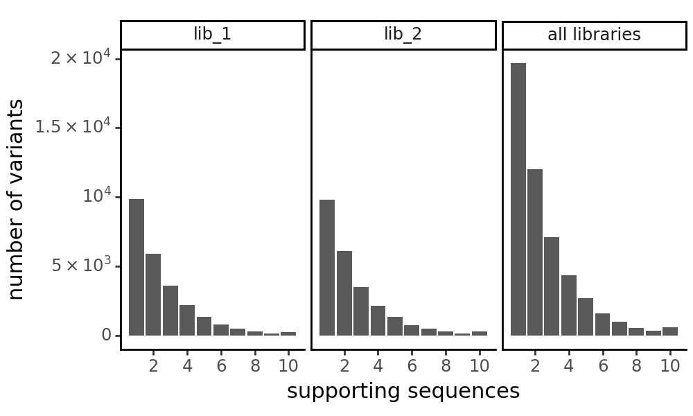
CodonVariantTable_h1.n_variants_df(samples=None)
[16]:
| library | sample | count | |
|---|---|---|---|
| 0 | lib_1 | barcoded variants | 25000 |
| 1 | lib_2 | barcoded variants | 25000 |
| 2 | all libraries | barcoded variants | 50000 |
plot the number of variant support sequences as a histogram
[17]:
p = CodonVariantTable_h1.plotVariantSupportHistogram(max_support=10)
p += theme_classic()
p += theme(
    panel_grid_major_x=element_blank(),  # no vertical grid lines
    figure_size=(5, 3)
)
_ = p.draw(show=True)

[18]:
CodonVariantTable_h2.n_variants_df(samples=None)
[18]:
| library | sample | count | |
|---|---|---|---|
| 0 | lib_1 | barcoded variants | 25000 |
| 1 | lib_2 | barcoded variants | 25000 |
| 2 | all libraries | barcoded variants | 50000 |
[19]:
p = CodonVariantTable_h2.plotVariantSupportHistogram(max_support=10)
p += theme_classic()
p += theme(
    panel_grid_major_x=element_blank(),  # no vertical grid lines
    figure_size=(5, 3)
)
_ = p.draw(show=True)
Variant phenotypes and enrichments
Now that we have simulated libraries of variants \(v_i \in V\), we’ll assign their respective ground truth phenotypes and enrichments.
We’ll start by computing latent phenotype, \(\phi(v_i)\). Recall that each of the two homologs has a SigmoidPhenotypeSimulator object that stores the latent effects of individual mutations. We will use these objects to compute the latent phenotypes of all variants in the libraries.
[20]:
# we'll store a collection of functions for each homolog
phenotype_fxn_dict_h1 = {"latentPhenotype" : SigmoidPhenotype_h1.latentPhenotype}
phenotype_fxn_dict_h2 = {"latentPhenotype" : SigmoidPhenotype_h2.latentPhenotype}

# add the latent phenotype to the barcode variant table
CodonVariantTable_h1.barcode_variant_df['latent_phenotype'] = CodonVariantTable_h1.barcode_variant_df['aa_substitutions'].apply(
    phenotype_fxn_dict_h1["latentPhenotype"]
)
CodonVariantTable_h2.barcode_variant_df['latent_phenotype'] = CodonVariantTable_h2.barcode_variant_df['aa_substitutions'].apply(
    phenotype_fxn_dict_h2["latentPhenotype"]
)

# print a sample of the variant table
CodonVariantTable_h1.barcode_variant_df[["library", "aa_substitutions", "latent_phenotype"]].head()
[20]:
| library | aa_substitutions | latent_phenotype | |
|---|---|---|---|
| 0 | lib_1 | V24Q S25R H27P D29L H33C S41L C44F S47F | -11.096139 |
| 1 | lib_1 | V8P H27T P30* L49P | -11.106200 |
| 2 | lib_1 | V19P V43Q | -2.878203 |
| 3 | lib_1 | R20Y | 5.161623 |
| 4 | lib_1 | 5.000000 |
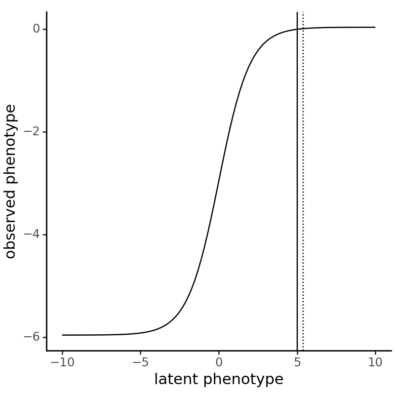
Next, we can compute an observed phenotype, \(p(v, d)\) = \(g_{\theta}(\phi(v, d))\), where \(g_{\theta}\) is the global epistasis function implimented as a flexible sigmoid with two free parameters, \(\theta_{s}\) and \(\theta_{b}\), that serve as a scale and bias, respectively. Concretely, \(g_{\theta}(z) = \theta_{b} + \frac{\theta_{s}}{1 + e^{-z}}\). For the purposes of this analysis, we compute a fixed value for the \(\theta_{b}\) parameter, based upon the
specified parameters for \(\theta_{s}\) (sigmoid_phenotype_scale) and \(\phi(v_{WT})\) (wt_latent) such that the reference wildtype phenotype is exactly 0.
Note that while the SigmoidPhenotypeSimulator object (as the name suggests) provides its own global epistasis object for computing phenotype and enrichments, we will only be using it to get mutational effects and the associated latent phenotypes. For computing the post-latent phenotypes and enrichments, we will use the multidms biophysical model such that we’re simulating under the same model we’ll be fitting as described above.
[21]:
# define numpy wrapper for multidms native jax sigmoid fxn
def g(z:float, ge_scale=sigmoid_phenotype_scale, wt_latent=wt_latent):

    # ensure the reference phenotype is 0
    ge_bias = -sigmoid_phenotype_scale / (1 + np.exp(-wt_latent))
    return ge_bias + (ge_scale/(1+np.exp(-z)))
Visualize the sigmoidal function that we’ll be using to map latent phenotypes to observed phenotypes. Place vertical line at the reference (“h1”) wildtype latent phenotype, as well as a dashed line for the non-reference (“h2”) phenotype:
[22]:
resolution = (-10, 10, 100)
p = (
    ggplot(
        pd.DataFrame(
            {
                "x":np.linspace(*resolution),
                "y":np.array(list(map(g, np.linspace(*resolution))))
            }
        ),
    )
    + geom_line(aes(x="x", y="y"))
    + geom_vline(xintercept=SigmoidPhenotype_h1.wt_latent)
    + geom_vline(xintercept=SigmoidPhenotype_h2.wt_latent, linetype="dotted")
    + labs(x="latent phenotype", y="observed phenotype")
    + theme_classic()
    + theme(figure_size=(4, 4))
)
_ = p.draw(show=True)
Next, assign each barcoded variant an observed phenotype, \(p(v, d)\), as well as an observed enrichment , \(2^{p(v, d)}\).
[23]:
subs = CodonVariantTable_h1.barcode_variant_df['aa_substitutions']
phenotype_fxn_dict_h1["observedPhenotype"] = lambda x: g(float(phenotype_fxn_dict_h1["latentPhenotype"](x)))
CodonVariantTable_h1.barcode_variant_df['observed_phenotype'] = subs.apply(
    phenotype_fxn_dict_h1["observedPhenotype"]
)
phenotype_fxn_dict_h1["observedEnrichment"] = lambda x: 2 ** (phenotype_fxn_dict_h1["observedPhenotype"](x))
CodonVariantTable_h1.barcode_variant_df['observed_enrichment'] = subs.apply(
    phenotype_fxn_dict_h1["observedEnrichment"]
)

subs = CodonVariantTable_h2.barcode_variant_df['aa_substitutions']
phenotype_fxn_dict_h2["observedPhenotype"] = lambda x: g(float(phenotype_fxn_dict_h2["latentPhenotype"](x)))
CodonVariantTable_h2.barcode_variant_df['observed_phenotype'] = subs.apply(
    phenotype_fxn_dict_h2["observedPhenotype"]
)
phenotype_fxn_dict_h2["observedEnrichment"] = lambda x: 2 ** (phenotype_fxn_dict_h2["observedPhenotype"](x))
CodonVariantTable_h2.barcode_variant_df['observed_enrichment'] = subs.apply(
    phenotype_fxn_dict_h2["observedEnrichment"]
)
variants_df = pd.concat(
    [
        CodonVariantTable_h1.barcode_variant_df.assign(homolog="h1"),
        CodonVariantTable_h2.barcode_variant_df.assign(homolog="h2")
    ]
)

variants_df[["aa_substitutions", "latent_phenotype", "observed_phenotype", "observed_enrichment", "homolog"]].head()
[23]:
| aa_substitutions | latent_phenotype | observed_phenotype | observed_enrichment | homolog | |
|---|---|---|---|---|---|
| 0 | V24Q S25R H27P D29L H33C S41L C44F S47F | -11.096139 | -5.959752 | 0.016067 | h1 |
| 1 | V8P H27T P30* L49P | -11.106200 | -5.959753 | 0.016067 | h1 |
| 2 | V19P V43Q | -2.878203 | -5.640393 | 0.020048 | h1 |
| 3 | R20Y | 5.161623 | 0.005959 | 1.004139 | h1 |
| 4 | 5.000000 | 0.000000 | 1.000000 | h1 |
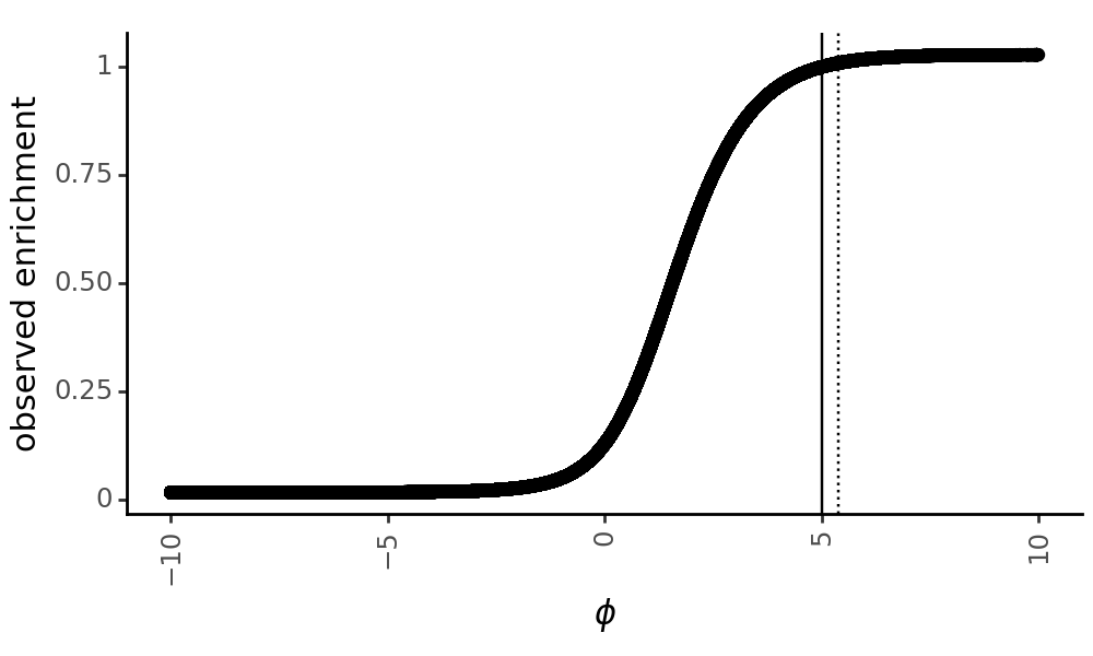
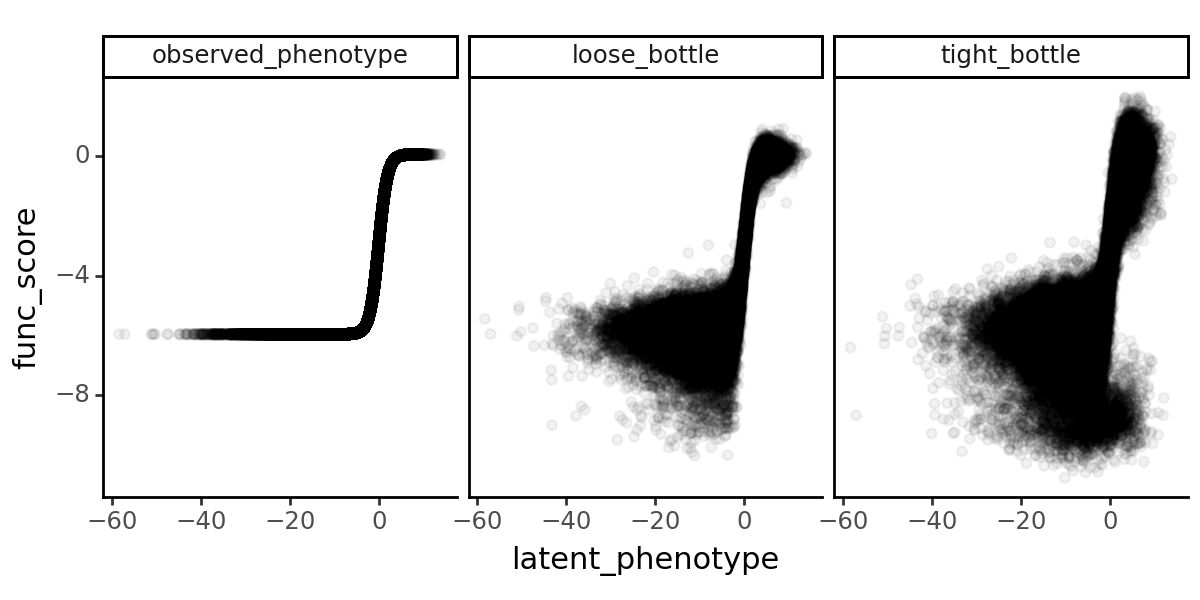
Note that The enrichment score transforms phenotypes to be between 0 and 1, and can thus be used to compute the number of counts for each variant in the post-selection library using a multinomial distribution where the probability of observing a variant is proportional to its enrichment. Below, we plot each variant’s latent phenotype against its observed enrichment:
[24]:
p = (
    ggplot(
        variants_df,
        aes(
            x = "latent_phenotype",
            y = "observed_enrichment"
        )
    )
    + geom_point()
    + geom_vline(xintercept=SigmoidPhenotype_h1.wt_latent)
    + geom_vline(xintercept=SigmoidPhenotype_h2.wt_latent, linetype="dotted")
    + theme_classic()
    + theme(
        figure_size=(5, 3),
        axis_text_x=element_text(angle=90),
        panel_grid_major_x=element_blank(),  # no vertical grid lines
    )
    + labs(
        x="$\phi$",
        y="observed enrichment"
    )
    # zoom in on the x axis limits
    + scale_x_continuous(limits=(-10, 10))
)
_ = p.draw(show=True)
Pre and post-selection variant read counts
Next, we will simulate both pre and post-selection counts of each variant subjected to an experimental selection step. Post-selection counts will be simulated by applying the specified selection bottleneck(s) to the pre-selection counts. To do this, we will use the functionality provided by dms_variants.simulate.simulateSampleCounts and feed it our custom phenotype function.
[25]:
bottlenecks = {
    name : variants_per_lib * scalar
    for name, scalar in bottleneck_variants_per_lib_scalar.items()
}

# do this independently for each of the homologs.
counts_h1, counts_h2 = [
    dms_variants.simulate.simulateSampleCounts(
        variants=variants,
        phenotype_func=pheno_fxn_dict["observedEnrichment"],
        variant_error_rate=variant_error_rate,
        pre_sample={
            "total_count": variants_per_lib * np.random.poisson(avgdepth_per_variant),
            "uniformity": lib_uniformity,
        },
        pre_sample_name="pre-selection",
        post_samples={
            name: {
                "noise": noise,
                "total_count": variants_per_lib * np.random.poisson(avgdepth_per_variant),
                "bottleneck": bottleneck,
            }
            for name, bottleneck in bottlenecks.items()
        },
        seed=seed,
    )
    for variants, pheno_fxn_dict in zip(
        [CodonVariantTable_h1, CodonVariantTable_h2], [phenotype_fxn_dict_h1, phenotype_fxn_dict_h2]
    )
]
CodonVariantTable_h1.add_sample_counts_df(counts_h1)
CodonVariantTable_h2.add_sample_counts_df(counts_h2)
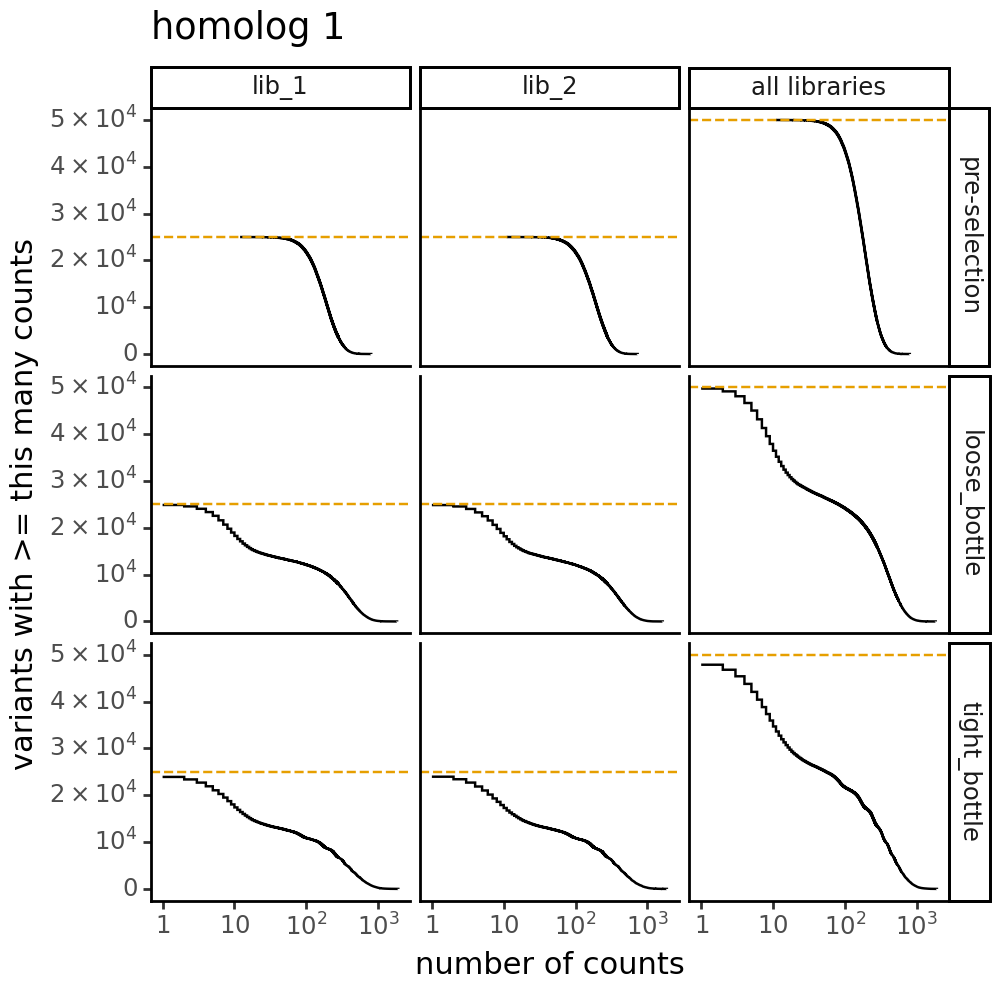
Plot the number of counts for each variant in each sample. The horizontal dashed line shows the total number of variants. The plot shows that all variants are well-sampled in the pre-selection libraries, but that post- selection some variants are sampled more or less. This is expected since selection will decrease and increase the frequency of variants:
[26]:
for variants, title in zip([CodonVariantTable_h1, CodonVariantTable_h2], ['homolog 1', 'homolog 2']):
    p = variants.plotCumulVariantCounts()
    p += theme_classic()
    p += theme(
        panel_grid_major_x=element_blank(),  # no vertical grid lines
        figure_size=(5, 5)
    )
    p += labs(title=title)
    _ = p.draw(show=True)

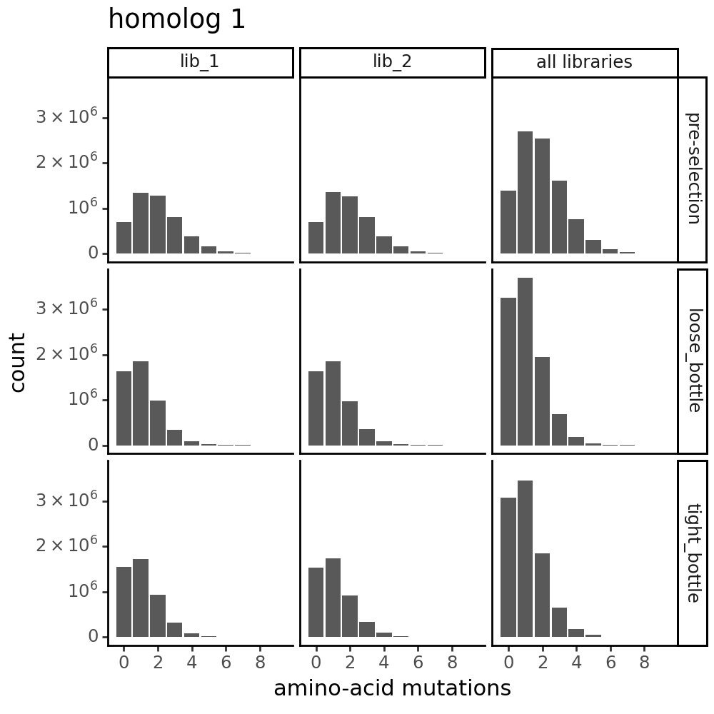
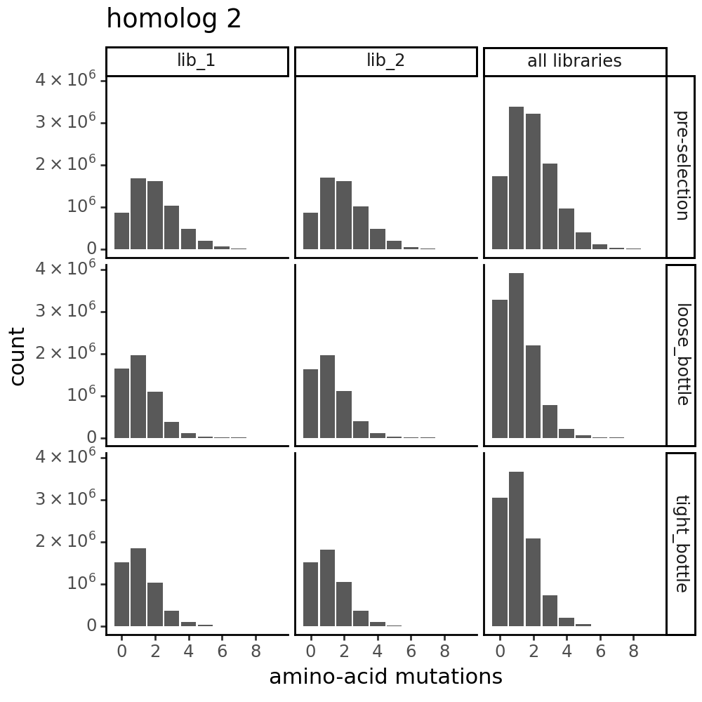
Distribution of the number of amino-acid mutations per variant in each sample. As expected, mutations go down after selection:
[27]:
for variants, title in zip([CodonVariantTable_h1, CodonVariantTable_h2], ['homolog 1', 'homolog 2']):
    p = variants.plotNumMutsHistogram(mut_type="aa")
    p += theme_classic()
    p += theme(figure_size=(5, 5))
    p += labs(title=title)
    _ = p.draw(show=True)
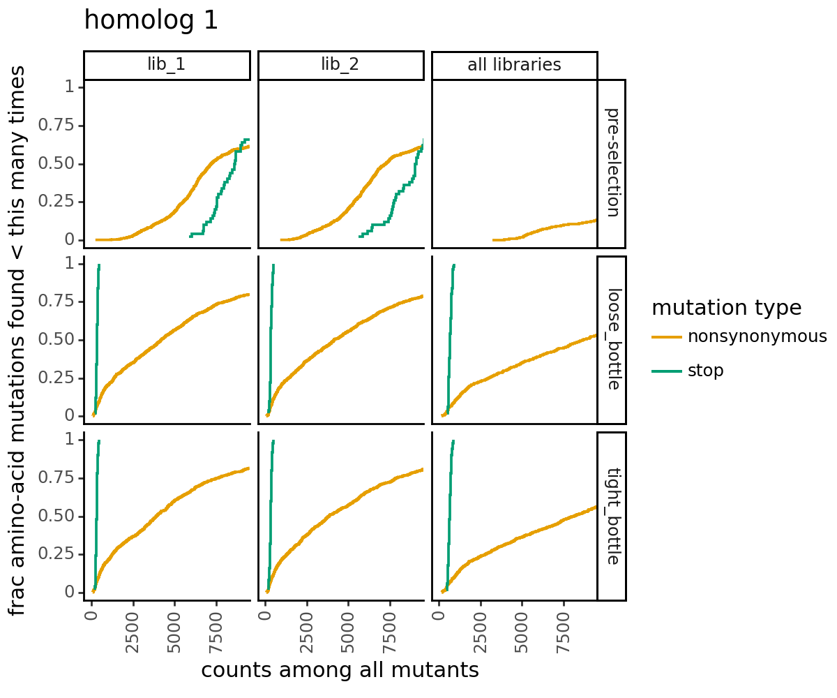
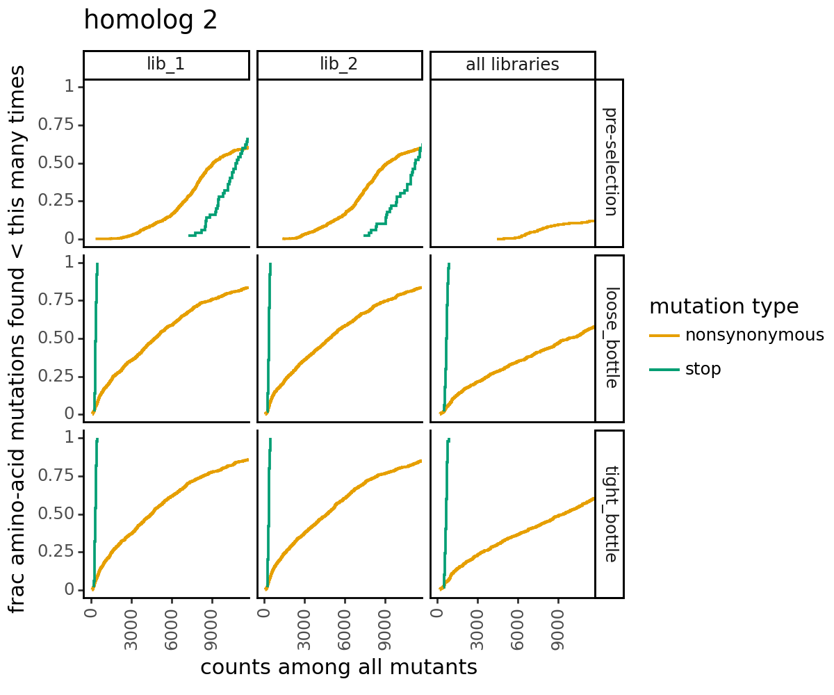
Plot how thoroughly amino-acid mutations are sampled. The plots below show that the stop mutations are sampled very poorly post-selection because they are eliminated during selection:
[28]:
for variants, title in zip([CodonVariantTable_h1, CodonVariantTable_h2], ['homolog 1', 'homolog 2']):
    p = variants.plotCumulMutCoverage(variant_type="all", mut_type="aa")
    p += theme_classic()
    p += theme(figure_size=(6, 5))
    p += theme(axis_text_x=element_text(angle=90))
    p += labs(title=title)
    _ = p.draw(show=True)
Prep training data
Prepare the training dataframes for fitting our multidms models.
As this is a joint-fitting approach, we combine homolog variants from each of the corresponding library replicates into a single training dataset. Additionally, for each replicate dataset, we’ll train models on each of the following targets representing different levels of noise in the data:
Ground truth observed phenotype - this target acts as a control and benchmarks the ability of the model to recover the true latent effects and shifts controlling for other sources of noise.
Loose bottleneck counts derived functional scores - these scores are derived from the observed enrichments, and used to asses model performance in the context of realistic experimental noise.
Tight bottleneck counts derived functional scores - the same as above, but with a tighter bottleneck for more extreme cases of noise.
For further details on how to prepare data and fit models, see the multidms quick-start tutorial.
Start by creating training data with ground truth phenotype target. Because the barcode replicates share ground truth phenotypes we can can collapse the counts accross replicates by simple dropping duplicates.
[29]:
req_cols = ["library", "homolog", "aa_substitutions", "func_score_type", "func_score"]
ground_truth_training_set = (
    pd.concat(
        [
            variants.barcode_variant_df[["library", "aa_substitutions", "observed_phenotype", "latent_phenotype"]]
            .drop_duplicates()
            .assign(homolog=homolog)
            for variants, homolog in zip([CodonVariantTable_h1, CodonVariantTable_h2], ['h1', 'h2'])
        ]
    )
    .melt(
        id_vars=["library", "aa_substitutions", "homolog", "latent_phenotype"],
        value_vars=["observed_phenotype"],
        var_name="func_score_type",
        value_name="func_score",
    )
    [req_cols]
    .astype({c:str for c in req_cols[:-1]})
)
ground_truth_training_set.round(2).head()
[29]:
| library | homolog | aa_substitutions | func_score_type | func_score | |
|---|---|---|---|---|---|
| 0 | lib_1 | h1 | V24Q S25R H27P D29L H33C S41L C44F S47F | observed_phenotype | -5.96 |
| 1 | lib_1 | h1 | V8P H27T P30* L49P | observed_phenotype | -5.96 |
| 2 | lib_1 | h1 | V19P V43Q | observed_phenotype | -5.64 |
| 3 | lib_1 | h1 | R20Y | observed_phenotype | 0.01 |
| 4 | lib_1 | h1 | observed_phenotype | 0.00 |
Next, compute functional scores from pre-post counts in each bottleneck after aggregating the barcode replicate counts for unique variants. The dms_variants.CodonVariantTable.func_scores method provides the ability to compute functional scores from pre and post-selection counts. We’ll use this to compute functional scores for each of the three targets:
[30]:
bottle_cbf = pd.concat(
    [
        (
            variants
            .func_scores("pre-selection", by="aa_substitutions", libraries=libs, syn_as_wt=True)
            .assign(homolog=homolog)
            .rename({"post_sample":"func_score_type"}, axis=1)
            [req_cols]
            .astype({c:str for c in req_cols[:-1]})
        )
        for variants, homolog in zip([CodonVariantTable_h1, CodonVariantTable_h2], ['h1', 'h2'])
    ]
)
bottle_cbf.head()
[30]:
| library | homolog | aa_substitutions | func_score_type | func_score | |
|---|---|---|---|---|---|
| 0 | lib_1 | h1 | Q28P | loose_bottle | -0.021369 |
| 1 | lib_1 | h1 | G50E | loose_bottle | -0.067491 |
| 2 | lib_1 | h1 | R48G | loose_bottle | -1.291522 |
| 3 | lib_1 | h1 | S3R G10Y L49H | loose_bottle | -5.759732 |
| 4 | lib_1 | h1 | F18T Q21E C44T | loose_bottle | -5.313711 |
Finally, combine the two dataframes computed above and classify the variants based on the number of amino acid substitutions.
[31]:
def classify_variant(aa_subs):
    if "*" in aa_subs:
        return "stop"
    elif aa_subs == "":
        return "wildtype"
    elif len(aa_subs.split()) == 1:
        return "1 nonsynonymous"
    elif len(aa_subs.split()) > 1:
        return ">1 nonsynonymous"
    else:
        raise ValueError(f"unexpected aa_subs: {aa_subs}")

func_scores = (
    pd.concat([ground_truth_training_set, bottle_cbf])
    .assign(variant_class = lambda x: x['aa_substitutions'].apply(classify_variant))
    .merge(
        variants_df[["aa_substitutions", "homolog", "latent_phenotype", "library"]].drop_duplicates(),
        on=["aa_substitutions", "homolog", "library"],
        how="inner"
    )
)

# categorical for plotting
func_scores["func_score_type"] = pd.Categorical(
    func_scores["func_score_type"],
    categories=["observed_phenotype", "loose_bottle", "tight_bottle"],
    ordered=True
)

func_scores
[31]:
| library | homolog | aa_substitutions | func_score_type | func_score | variant_class | latent_phenotype | |
|---|---|---|---|---|---|---|---|
| 0 | lib_1 | h1 | V24Q S25R H27P D29L H33C S41L C44F S47F | observed_phenotype | -5.959752 | >1 nonsynonymous | -11.096139 |
| 1 | lib_1 | h1 | V8P H27T P30* L49P | observed_phenotype | -5.959753 | stop | -11.106200 |
| 2 | lib_1 | h1 | V19P V43Q | observed_phenotype | -5.640393 | >1 nonsynonymous | -2.878203 |
| 3 | lib_1 | h1 | R20Y | observed_phenotype | 0.005959 | 1 nonsynonymous | 5.161623 |
| 4 | lib_1 | h1 | observed_phenotype | 0.000000 | wildtype | 5.000000 | |
| ... | ... | ... | ... | ... | ... | ... | ... |
| 181363 | lib_2 | h2 | E9L Q21L V24Q S25V D29V D38Q | tight_bottle | -6.184609 | >1 nonsynonymous | -11.209818 |
| 181364 | lib_2 | h2 | S47T V49E | tight_bottle | 1.125946 | >1 nonsynonymous | 3.861711 |
| 181365 | lib_2 | h2 | G10P I35S G50L | tight_bottle | -3.634411 | >1 nonsynonymous | -12.580142 |
| 181366 | lib_2 | h2 | F15R I35S D38E Y39G | tight_bottle | -5.781253 | >1 nonsynonymous | -15.097683 |
| 181367 | lib_2 | h2 | E9F C34P Y39C E44Y T45F | tight_bottle | -5.581944 | >1 nonsynonymous | -6.628840 |
181368 rows × 7 columns
Let’s plot the functional scores as a function of the latent phenotype.
[32]:
p = (
    ggplot(func_scores, aes(x="latent_phenotype", y="func_score"))
    + geom_point(alpha=0.05)
    + facet_wrap("~func_score_type")
    + theme_classic()
    + theme(figure_size=(6, 3))
)
_ = p.draw(show=True)
Plot a pairplot to see how targets compare.
[33]:
fig = sns.pairplot(
    (
        func_scores
        .pivot(
            index=["library", "homolog", "aa_substitutions", "variant_class"],
            columns="func_score_type",
            values="func_score"
        )
        .reset_index()
        .sample(frac=0.1)
    ),
    hue='homolog',
    plot_kws = {"alpha":0.25},
    corner=True
)
fig.fig.set_size_inches(6, 5)
plt.tight_layout()
plt.show()
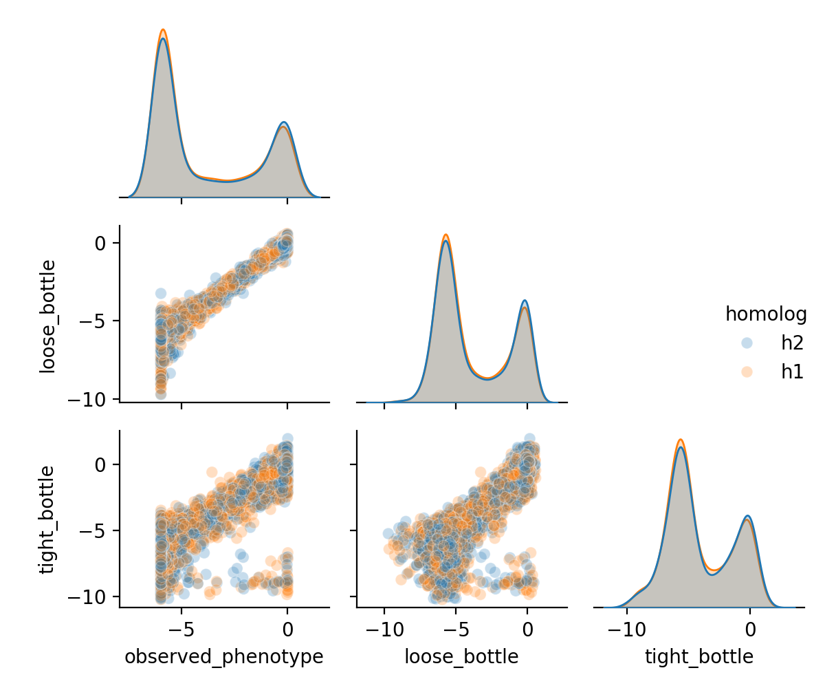
We can see here that the tight bottleneck indeed introduces more noise in the data, as the functional scores are less correlated with the ground truth phenotype.
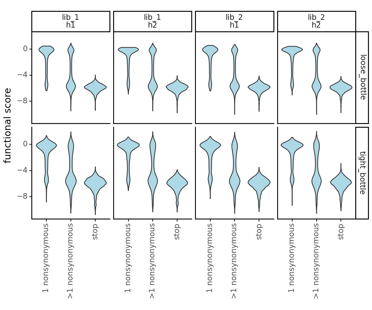
Plot the functional scores distributions of the bottleneck counts-computed functional scores. Recall that we collapsed barcode replicates so there is only a single wildtype phenotype in each of the datasets, thus we will not plot them below.
[34]:
p = (
    ggplot(
        func_scores.query("(func_score_type != 'observed_phenotype') & (variant_class != 'wildtype')"),
        aes("variant_class", "func_score")
    )
    + geom_violin(fill="lightblue")
    + ylab("functional score")
    + xlab("")
    + facet_grid("func_score_type ~ library + homolog")
    + theme_classic()
    + theme(
        figure_size=(6, 5),
        axis_text_x=element_text(angle=90),
        panel_grid_major_x=element_blank(),  # no vertical grid lines
    )
    # + scale_fill_manual(values=CBPALETTE[1:])
)
_ = p.draw(show=True)
[35]:
func_scores.to_csv(f"{csv_output_dir}/simulated_func_scores.csv", index=False)
func_scores.round(2).head()
[35]:
| library | homolog | aa_substitutions | func_score_type | func_score | variant_class | latent_phenotype | |
|---|---|---|---|---|---|---|---|
| 0 | lib_1 | h1 | V24Q S25R H27P D29L H33C S41L C44F S47F | observed_phenotype | -5.96 | >1 nonsynonymous | -11.10 |
| 1 | lib_1 | h1 | V8P H27T P30* L49P | observed_phenotype | -5.96 | stop | -11.11 |
| 2 | lib_1 | h1 | V19P V43Q | observed_phenotype | -5.64 | >1 nonsynonymous | -2.88 |
| 3 | lib_1 | h1 | R20Y | observed_phenotype | 0.01 | 1 nonsynonymous | 5.16 |
| 4 | lib_1 | h1 | observed_phenotype | 0.00 | wildtype | 5.00 |
Create Data objects for each library replicate, and bottleneck
multidms model fitting is generally a two-step process: (1) Create Data objects from functional score dataframes which, among other things, encode the variant data into one-hot encoded matrices, and (2) fit a collection of models across a grid of Data objects and hyperparameters. Here, we’ll create Data objects for each library replicate / fitting target combination:
[36]:
data_objects = [
    multidms.Data(
        fs_df,
        reference="h1",
        alphabet = multidms.AAS_WITHSTOP_WITHGAP,
        verbose=False,
        name = f"{lib}_{target}_func_score"
    )
    for (lib, target), fs_df in func_scores.rename(columns={"homolog":"condition"}).groupby(['library', 'func_score_type'])
]

data_objects
[36]:
[Data(lib_1_observed_phenotype_func_score),
 Data(lib_1_loose_bottle_func_score),
 Data(lib_1_tight_bottle_func_score),
 Data(lib_2_observed_phenotype_func_score),
 Data(lib_2_loose_bottle_func_score),
 Data(lib_2_tight_bottle_func_score)]
Fit models to training data (lasso sweep)
Next, we’ll fit a set of models to each of the datasets defined above using the multidms.fit_models function. For each dataset, we independently fit models with a number of different lasso penalty coefficients (\(\lambda_{L1}\)) as defined at the top of this notebook.
[115]:
fitting_params = {
    # "num_training_steps": [num_training_steps], # default 100
    "maxiter": [10000], # default 20000
    "tol":[0.0001],
    "scale_coeff_lasso_shift": scale_coeff_lasso_shift, # the sweep of lasso coefficient params
    "init_beta_naught" : [init_beta_naught], # We've found that we need to start with a higher beta_naught to get the model to converge correctly,
    "scale_coeff_ridge_beta" : [scale_coeff_ridge_beta], # the sweep of ridge coefficient params
    "acceleration" : [True], # default True
    "maxls" : [50]
}

fitting_params["dataset"] = data_objects
pprint.pprint(fitting_params)
{'acceleration': [True],
 'dataset': [Data(lib_1_observed_phenotype_func_score),
             Data(lib_1_loose_bottle_func_score),
             Data(lib_1_tight_bottle_func_score),
             Data(lib_2_observed_phenotype_func_score),
             Data(lib_2_loose_bottle_func_score),
             Data(lib_2_tight_bottle_func_score)],
 'init_beta_naught': [5.0],
 'maxiter': [10000],
 'maxls': [50],
 'scale_coeff_lasso_shift': [0.0,
                             5e-06,
                             1e-05,
                             2e-05,
                             4e-05,
                             8e-05,
                             0.00016,
                             0.00032,
                             0.00064],
 'scale_coeff_ridge_beta': [1e-07],
 'tol': [0.0001]}
[116]:
pprint.pprint(multidms.model_collection._explode_params_dict(fitting_params)[0])
{'acceleration': True,
 'dataset': Data(lib_1_observed_phenotype_func_score),
 'init_beta_naught': 5.0,
 'maxiter': 10000,
 'maxls': 50,
 'scale_coeff_lasso_shift': 0.0,
 'scale_coeff_ridge_beta': 1e-07,
 'tol': 0.0001}
[117]:
multidms.model_collection.fit_one_model(**multidms.model_collection._explode_params_dict(fitting_params)[0])
---------------------------------------------------------------------------
KeyError                                  Traceback (most recent call last)
/home/jgallowa/Projects/multidms/notebooks/simulation_validation.ipynb Cell 90 line 1
----> <a href='vscode-notebook-cell://ssh-remote%2Bermine.fhcrc.org/home/jgallowa/Projects/multidms/notebooks/simulation_validation.ipynb#Y316sdnNjb2RlLXJlbW90ZQ%3D%3D?line=0'>1</a> multidms.model_collection.fit_one_model(**multidms.model_collection._explode_params_dict(fitting_params)[0])

File ~/Projects/multidms/multidms/model_collection.py:245, in fit_one_model(dataset, epistatic_model, output_activation, lock_beta_naught_at, gamma_corrected, alpha_d, init_beta_naught, n_hidden_units, lower_bound, PRNGKey, verbose, **kwargs)
    221 fit_attributes["fit_time"] = round(end - start)
    223 col_order = [
    224     "model",
    225     "dataset_name",
   (...)
    242     "PRNGKey",
    243 ]
--> 245 return pd.Series(fit_attributes)[col_order]

File ~/mambaforge/envs/multidms-dev/lib/python3.11/site-packages/pandas/core/series.py:1144, in Series.__getitem__(self, key)
   1141     key = np.asarray(key, dtype=bool)
   1142     return self._get_rows_with_mask(key)
-> 1144 return self._get_with(key)

File ~/mambaforge/envs/multidms-dev/lib/python3.11/site-packages/pandas/core/series.py:1185, in Series._get_with(self, key)
   1182         return self.iloc[key]
   1184 # handle the dup indexing case GH#4246
-> 1185 return self.loc[key]

File ~/mambaforge/envs/multidms-dev/lib/python3.11/site-packages/pandas/core/indexing.py:1191, in _LocationIndexer.__getitem__(self, key)
   1189 maybe_callable = com.apply_if_callable(key, self.obj)
   1190 maybe_callable = self._check_deprecated_callable_usage(key, maybe_callable)
-> 1191 return self._getitem_axis(maybe_callable, axis=axis)

File ~/mambaforge/envs/multidms-dev/lib/python3.11/site-packages/pandas/core/indexing.py:1420, in _LocIndexer._getitem_axis(self, key, axis)
   1417     if hasattr(key, "ndim") and key.ndim > 1:
   1418         raise ValueError("Cannot index with multidimensional key")
-> 1420     return self._getitem_iterable(key, axis=axis)
   1422 # nested tuple slicing
   1423 if is_nested_tuple(key, labels):

File ~/mambaforge/envs/multidms-dev/lib/python3.11/site-packages/pandas/core/indexing.py:1360, in _LocIndexer._getitem_iterable(self, key, axis)
   1357 self._validate_key(key, axis)
   1359 # A collection of keys
-> 1360 keyarr, indexer = self._get_listlike_indexer(key, axis)
   1361 return self.obj._reindex_with_indexers(
   1362     {axis: [keyarr, indexer]}, copy=True, allow_dups=True
   1363 )

File ~/mambaforge/envs/multidms-dev/lib/python3.11/site-packages/pandas/core/indexing.py:1558, in _LocIndexer._get_listlike_indexer(self, key, axis)
   1555 ax = self.obj._get_axis(axis)
   1556 axis_name = self.obj._get_axis_name(axis)
-> 1558 keyarr, indexer = ax._get_indexer_strict(key, axis_name)
   1560 return keyarr, indexer

File ~/mambaforge/envs/multidms-dev/lib/python3.11/site-packages/pandas/core/indexes/base.py:6200, in Index._get_indexer_strict(self, key, axis_name)
   6197 else:
   6198     keyarr, indexer, new_indexer = self._reindex_non_unique(keyarr)
-> 6200 self._raise_if_missing(keyarr, indexer, axis_name)
   6202 keyarr = self.take(indexer)
   6203 if isinstance(key, Index):
   6204     # GH 42790 - Preserve name from an Index

File ~/mambaforge/envs/multidms-dev/lib/python3.11/site-packages/pandas/core/indexes/base.py:6252, in Index._raise_if_missing(self, key, indexer, axis_name)
   6249     raise KeyError(f"None of [{key}] are in the [{axis_name}]")
   6251 not_found = list(ensure_index(key)[missing_mask.nonzero()[0]].unique())
-> 6252 raise KeyError(f"{not_found} not in index")

KeyError: "['scale_coeff_lasso_shift', 'scale_coeff_ridge_beta', 'scale_coeff_ridge_shift', 'scale_coeff_ridge_gamma', 'scale_coeff_ridge_alpha_d', 'huber_scale_huber', 'tol', 'maxiter'] not in index"
Fit the models:
[112]:
_, _, fit_collection_df = multidms.model_collection.fit_models(fitting_params)
Note that the return type of multidms.fit_models is a tuple(int, int, pd.DataFrame) where the first two values are the number of fits that were successful and the number that failed, respectively, and the third value is a dataframe where each row contains a fit Model object and the hyperparameters used to fit it.
[107]:
fit_collection_df[["model", "dataset_name", "scale_coeff_lasso_shift", "fit_time"]].info()
<class 'pandas.core.frame.DataFrame'>
RangeIndex: 108 entries, 0 to 107
Data columns (total 4 columns):
 #   Column                   Non-Null Count  Dtype
---  ------                   --------------  -----
 0   model                    108 non-null    object
 1   dataset_name             108 non-null    object
 2   scale_coeff_lasso_shift  108 non-null    object
 3   fit_time                 108 non-null    object
dtypes: object(4)
memory usage: 3.5+ KB
Add a few helpful features to this dataframe for plotting by splitting the “dataset_name” (name of the Data Object that was used for fitting) into more understandable columns:
[78]:
fit_collection_df = fit_collection_df.assign(
    measurement_type = fit_collection_df["dataset_name"].str.split("_").str[2:4].str.join("_"),
    library = fit_collection_df["dataset_name"].str.split("_").str[0:2].str.join("_")
)

# convert measurement type to categorical ordered by 'observed', 'loose', 'tight' for plotting
fit_collection_df["measurement_type"] = pd.Categorical(
    fit_collection_df["measurement_type"],
    categories=["observed_phenotype", "loose_bottle", "tight_bottle"],
    ordered=True
)

fit_collection_df[["model", "measurement_type", "library", "scale_coeff_lasso_shift"]].head()
[78]:
| model | measurement_type | library | scale_coeff_lasso_shift | |
|---|---|---|---|---|
| 0 | Model(Model-0) | observed_phenotype | lib_1 | 0.0 |
| 1 | Model(Model-0) | observed_phenotype | lib_1 | 0.000005 |
| 2 | Model(Model-0) | observed_phenotype | lib_1 | 0.00001 |
| 3 | Model(Model-0) | observed_phenotype | lib_1 | 0.00002 |
| 4 | Model(Model-0) | observed_phenotype | lib_1 | 0.00004 |
Model convergence
[79]:
# %load_ext autoreload
# %autoreload 2

# import multidms
[121]:
# model_collection_100K_50_w_wo_acceleration = model_collection
model_collection = model_collection_100K_50_w_wo_acceleration
[119]:
model_collection = multidms.model_collection.ModelCollection(fit_collection_df)
model_collection.fit_models.converged.value_counts()
[119]:
converged
False    54
Name: count, dtype: int64
[122]:
data = model_collection.convergence_trajectory_df(
    id_vars = ("scale_coeff_lasso_shift", "measurement_type", "library", "acceleration", "maxls")
)
data
[122]:
| loss | error | scale_coeff_lasso_shift | measurement_type | library | acceleration | maxls | |
|---|---|---|---|---|---|---|---|
| step | |||||||
| 0 | 6.365419 | inf | 0.00000 | observed_phenotype | lib_1 | True | 50 |
| 100 | 3.200364 | 0.053223 | 0.00000 | observed_phenotype | lib_1 | True | 50 |
| 200 | 1.740282 | 3.078689 | 0.00000 | observed_phenotype | lib_1 | True | 50 |
| 300 | 0.424062 | 0.927919 | 0.00000 | observed_phenotype | lib_1 | True | 50 |
| 400 | 0.124201 | 1.327493 | 0.00000 | observed_phenotype | lib_1 | True | 50 |
| ... | ... | ... | ... | ... | ... | ... | ... |
| 99600 | 0.859699 | 0.001236 | 0.00064 | tight_bottle | lib_2 | False | 50 |
| 99700 | 0.859631 | 0.001307 | 0.00064 | tight_bottle | lib_2 | False | 50 |
| 99800 | 0.859563 | 0.000868 | 0.00064 | tight_bottle | lib_2 | False | 50 |
| 99900 | 0.859490 | 0.001191 | 0.00064 | tight_bottle | lib_2 | False | 50 |
| 100000 | 0.859420 | 0.001040 | 0.00064 | tight_bottle | lib_2 | False | 50 |
108108 rows × 7 columns
[123]:
data.index.name = "step"
data.reset_index(inplace=True)
data.head()
[123]:
| step | loss | error | scale_coeff_lasso_shift | measurement_type | library | acceleration | maxls | |
|---|---|---|---|---|---|---|---|---|
| 0 | 0 | 6.365419 | inf | 0.0 | observed_phenotype | lib_1 | True | 50 |
| 1 | 100 | 3.200364 | 0.053223 | 0.0 | observed_phenotype | lib_1 | True | 50 |
| 2 | 200 | 1.740282 | 3.078689 | 0.0 | observed_phenotype | lib_1 | True | 50 |
| 3 | 300 | 0.424062 | 0.927919 | 0.0 | observed_phenotype | lib_1 | True | 50 |
| 4 | 400 | 0.124201 | 1.327493 | 0.0 | observed_phenotype | lib_1 | True | 50 |
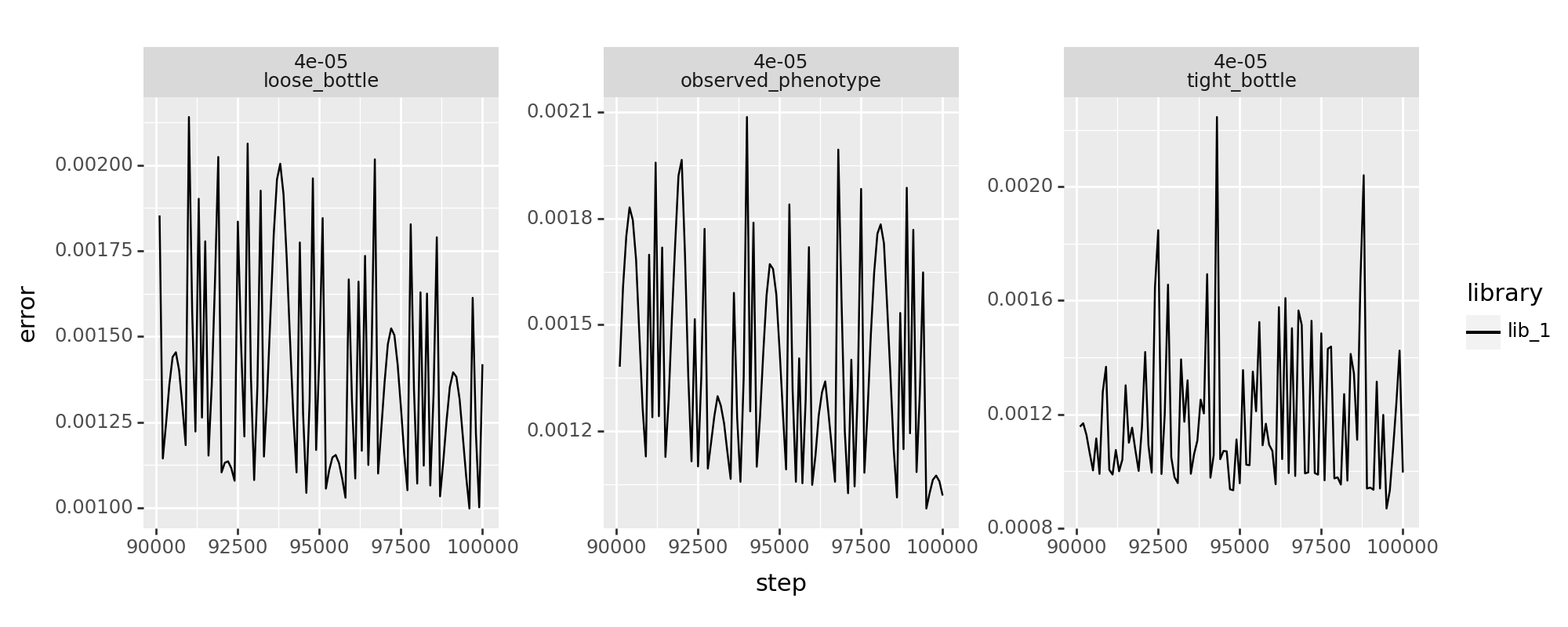
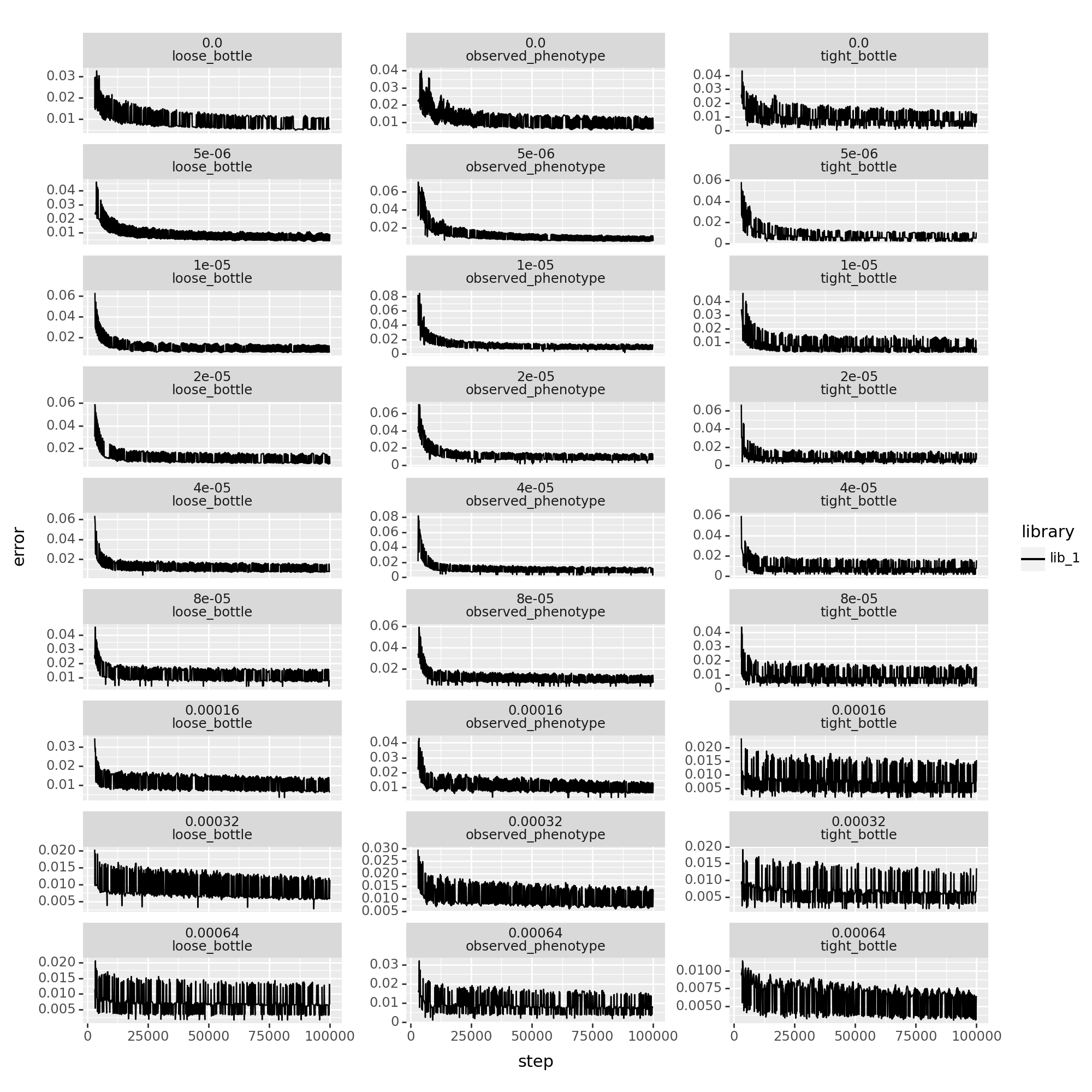
[133]:
p = (
    ggplot(
        data.query("~acceleration & step > 90000 & library == 'lib_1' & scale_coeff_lasso_shift == 4e-05"),
        aes(
            x="step",
            y="error",
            linetype="library"
        )
    )
    + geom_line()
    + facet_wrap("~scale_coeff_lasso_shift+measurement_type", scales="free_y", ncol=3)
    # copnstrain y axis to 0-1
    # + scale_y_continuous(limits=(0, .1))
    # make figure size taller
    + theme(figure_size=(10, 4))
    # add title
    + labs(
        # title="acceleration=False"
    )
)
_ = p.draw(show=True)
[135]:
p = (
    ggplot(
        data.query("acceleration & step > 3000 & library == 'lib_1'"),
        aes(
            x="step",
            y="error",
            linetype="library"
        )
    )
    + geom_line()
    + facet_wrap("~scale_coeff_lasso_shift+measurement_type", scales="free_y", ncol=3)
    # copnstrain y axis to 0-1
    # + scale_y_continuous(limits=(0, .1))
    # make figure size taller
    + theme(figure_size=(10, 10))
)
_ = p.draw(show=True)
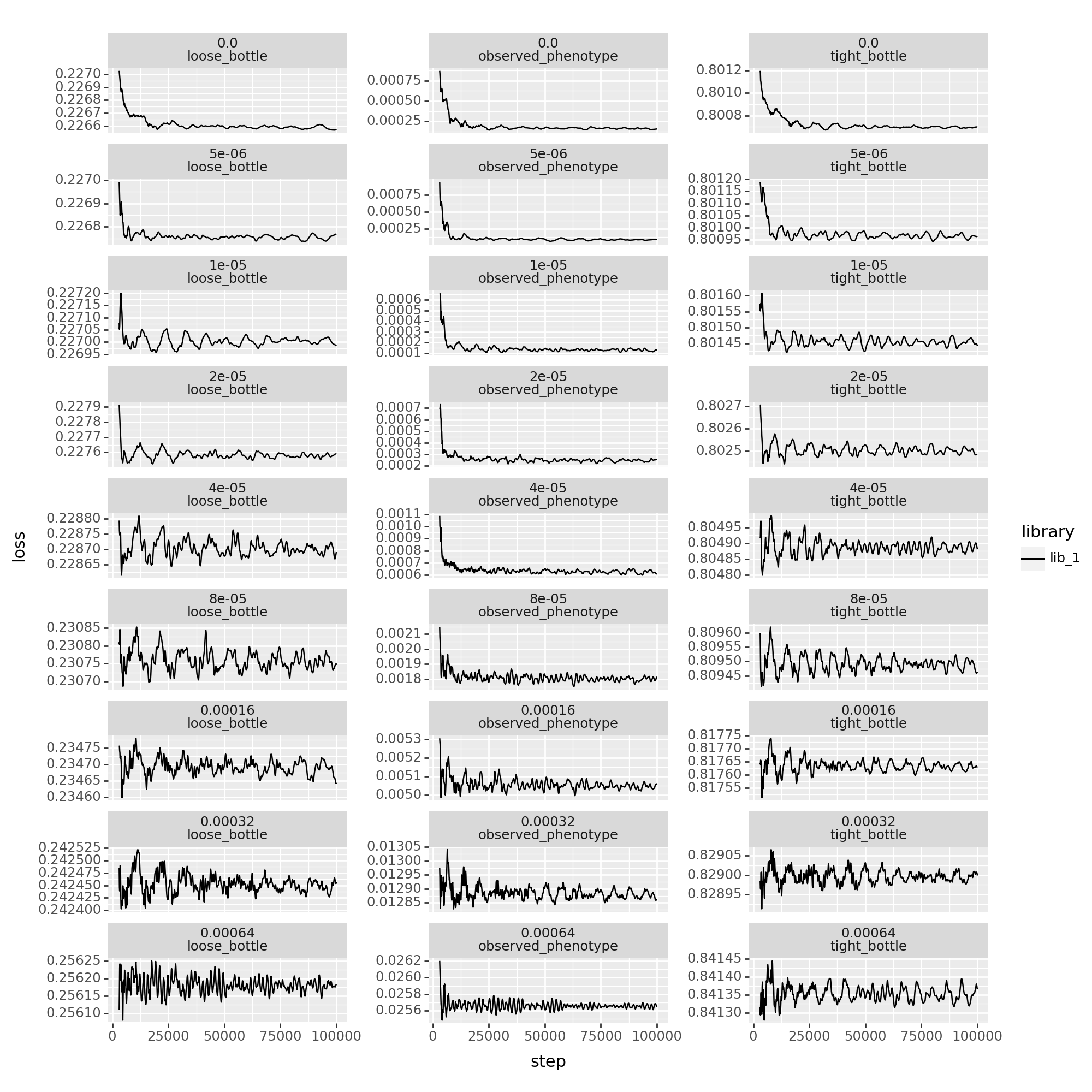
[ ]:
p = (
    ggplot(
        data.query("acceleration & step > 3000 & library == 'lib_1'"),
        aes(
            x="step",
            y="loss",
            linetype="library"
        )
    )
    + geom_line()
    + facet_wrap("~scale_coeff_lasso_shift+measurement_type", scales="free_y", ncol=3)
    # copnstrain y axis to 0-1
    # + scale_y_continuous(limits=(0, .1))
    # make figure size taller
    + theme(figure_size=(10, 10))
)
_ = p.draw(show=True)
Model vs. truth mutational effects
The multidms.ModelCollection takes a a dataframe such as the one created above and provides a few helpful methods for model selection and aggregation. We’ll use these methods to evaluate the fits and select the best model for each dataset.
[42]:
model_collection = multidms.model_collection.ModelCollection(fit_collection_df)
[43]:
model_collection.fit_models.converged.value_counts()
[43]:
converged
False    54
Name: count, dtype: int64
[46]:
chart_no_bottle = model_collection.mut_param_dataset_correlation(query="measurement_type == 'observed_phenotype'")
chart_loose_bottle = model_collection.mut_param_dataset_correlation(query="measurement_type == 'loose_bottle'")
chart_tight_bottle = model_collection.mut_param_dataset_correlation(query="measurement_type == 'tight_bottle'")
chart_no_bottle | chart_loose_bottle | chart_tight_bottle
cache miss - this could take a moment
cache miss - this could take a moment
[46]:
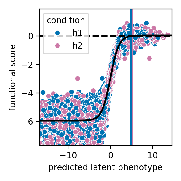
[48]:
(
    model_collection
    .fit_models
    .query(
        f"scale_coeff_lasso_shift == 8.0e-5 and measurement_type == 'loose_bottle' and library == 'lib_1'"
    )
    .iloc[0]
    .model
    .plot_epistasis()
)
[48]:
<Axes: xlabel='predicted latent phenotype', ylabel='functional score'>
Get the mutational parameters for each of the models using model_collection.split_apply_combine_muts() method, and merge them with the simulated ground truth parameters:
[42]:
# the columns that distinguish fits are what we'll groupby such that none of the model collection parameters are aggregated
groupby=("library", "measurement_type", "scale_coeff_lasso_shift")
collection_muts_df = (
    model_collection.split_apply_combine_muts(
        groupby=groupby
    )
    .reset_index()
    .rename(
        {
            'beta' : 'predicted_beta',
            'shift_h2' : 'predicted_shift_h2',
        },
        axis=1
    )
    .merge(
        mut_effects_df.rename(
            {
                'beta_h1' : 'true_beta',
                'beta_h2' : 'true_beta_h2',
                'shift' : 'true_shift',
            },
            axis=1
        ),
        on='mutation'
    )
)
assert collection_muts_df.shape[0] == len(mut_effects_df) * len(fit_collection_df)
collection_muts_df[["mutation", "library", "measurement_type", "scale_coeff_lasso_shift", "predicted_shift_h2", "true_shift"]].head()
cache miss - this could take a moment
[42]:
| mutation | library | measurement_type | scale_coeff_lasso_shift | predicted_shift_h2 | true_shift | |
|---|---|---|---|---|---|---|
| 0 | C31* | lib_1 | observed_phenotype | 0.0 | -15.289572 | 0.0 |
| 1 | C31A | lib_1 | observed_phenotype | 0.0 | -0.003453 | 0.0 |
| 2 | C31D | lib_1 | observed_phenotype | 0.0 | -0.030438 | 0.0 |
| 3 | C31E | lib_1 | observed_phenotype | 0.0 | -0.086455 | 0.0 |
| 4 | C31F | lib_1 | observed_phenotype | 0.0 | -0.021350 | 0.0 |
To compare model fits parameter values to the simulated ground truth values, add mean squared error and pearsonr metrics to the ModelCollection.fit_models attribute:
[43]:
def series_corr(y_true, y_pred):
    return np.corrcoef(y_true, y_pred)[0, 1]

def series_mae(y_true, y_pred):
    return np.mean(y_true - y_pred)

# compute the new metric columns
new_fit_models_cols = defaultdict(list)
for group, model_mutations_df in collection_muts_df.groupby(list(groupby)):
    # add cols for merging
    for i, attribute in enumerate(group):
        new_fit_models_cols[groupby[i]].append(group[i])

    for parameter in ["beta", "shift"]:
        for metric_fxn, name in zip([series_corr, series_mae], ["corr", "mae"]):

            # add the new metric columns
            postfix="_h2" if parameter == "shift" else ""
            y_pred = model_mutations_df[f"predicted_{parameter}{postfix}"]
            y_true = model_mutations_df[f"true_{parameter}"]
            new_fit_models_cols[f"{parameter}_{name}"].append(metric_fxn(y_true, y_pred))

# merge the new columns into the model collection
model_collection.fit_models = model_collection.fit_models.merge(
    pd.DataFrame(new_fit_models_cols),
    on=list(groupby)
)

# print the first few rows of the model collection
model_collection.fit_models[list(groupby) + [c for c in new_fit_models_cols.keys() if c not in groupby]].head()
[43]:
| library | measurement_type | scale_coeff_lasso_shift | beta_corr | beta_mae | shift_corr | shift_mae | |
|---|---|---|---|---|---|---|---|
| 0 | lib_1 | observed_phenotype | 0.0 | 0.977246 | -0.268842 | 0.109992 | 1.172704 |
| 1 | lib_1 | observed_phenotype | 0.000005 | 0.985431 | -0.206331 | 0.997367 | 0.000190 |
| 2 | lib_1 | observed_phenotype | 0.00001 | 0.984181 | -0.217609 | 0.994465 | -0.000601 |
| 3 | lib_1 | observed_phenotype | 0.00002 | 0.984685 | -0.220858 | 0.990086 | -0.000248 |
| 4 | lib_1 | observed_phenotype | 0.00004 | 0.984756 | -0.226117 | 0.979619 | 0.001351 |
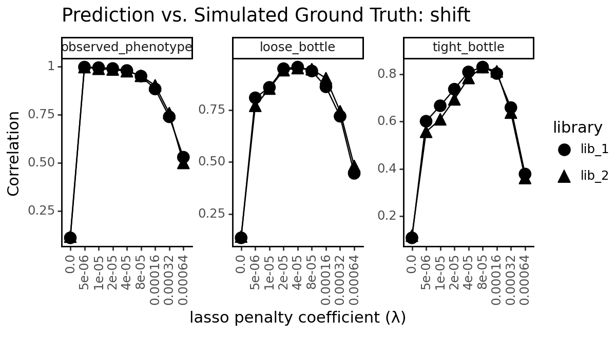
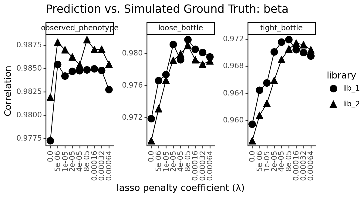
Next, we’ll make some summary plots with the predicted vs. simulated ground MSE truth parameters across model fits
[44]:
metric = "corr"

data = (
    model_collection.fit_models
    .assign(
        measurement_library = lambda x: x["measurement_type"].astype(str) + " " + x["library"]
    )
    .melt(
        id_vars=list(groupby) + ["measurement_library"],
        value_vars=[f"beta_{metric}", f"shift_{metric}"],
        var_name="parameter",
        value_name=metric,
    )
)
data["measurement_type"] = pd.Categorical(
    data["measurement_type"],
    categories=["observed_phenotype", "loose_bottle", "tight_bottle"],
    ordered=True
)
data["parameter"] = data["parameter"].str.replace(f"_{metric}", "")
data["parameter"] = pd.Categorical(
    data["parameter"],
    categories=["shift", "beta"],
    ordered=True
)
for parameter, parameter_df in data.groupby("parameter", observed=True):
    p = (
        ggplot(parameter_df)
        + geom_line(
            aes(
                x="scale_coeff_lasso_shift",
                y=metric,
                group="measurement_library",
            ),
        )
        + geom_point(
            aes(
                x="scale_coeff_lasso_shift",
                y=metric,
                shape="library"
            ),
            size=4
        )
        + facet_wrap("measurement_type", scales="free_y")
        + theme_classic()
        + theme(
            figure_size=(6, 3.3),
            axis_text_x=element_text(angle=90),
            panel_grid_major_x=element_blank(),  # no vertical grid lines
        )
        + labs(
            title=f"Prediction vs. Simulated Ground Truth: {parameter}",
            x="lasso penalty coefficient (λ)",
            y="Mean Absolute Error" if metric == "mae" else "Correlation"
        )
    )
    _ = p.draw(show=True)
[45]:
data.to_csv(f"{csv_output_dir}/model_vs_truth_beta_shift.csv", index=False)
data.round(2).head()
[45]:
| library | measurement_type | scale_coeff_lasso_shift | measurement_library | parameter | corr | |
|---|---|---|---|---|---|---|
| 0 | lib_1 | observed_phenotype | 0.0 | observed_phenotype lib_1 | beta | 0.98 |
| 1 | lib_1 | observed_phenotype | 0.000005 | observed_phenotype lib_1 | beta | 0.99 |
| 2 | lib_1 | observed_phenotype | 0.00001 | observed_phenotype lib_1 | beta | 0.98 |
| 3 | lib_1 | observed_phenotype | 0.00002 | observed_phenotype lib_1 | beta | 0.98 |
| 4 | lib_1 | observed_phenotype | 0.00004 | observed_phenotype lib_1 | beta | 0.98 |
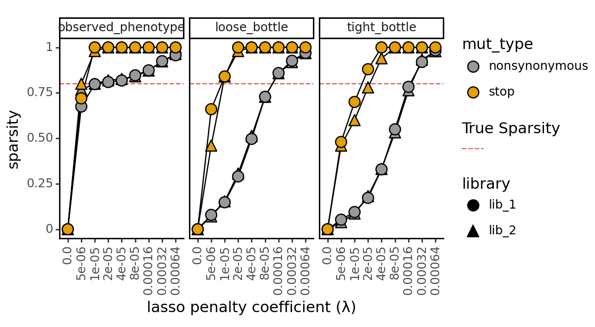
Shift sparsity
Another way we might evaluate the fits is by looking at the sparsity of the models by computing the percentage of shift parameters that are equal to zero among the models. We look at this metric separately for mutations to stop codons and mutations to non-stop codons because we expect the stop codons to be equally deleterious in both homologs, and thus we expect all the shift parameters associated with stop codon mutations to be zero in a “good” fit.
[46]:
chart, data = model_collection.shift_sparsity(return_data=True)
data.head()
cache miss - this could take a moment
[46]:
| dataset_name | scale_coeff_lasso_shift | mut_type | mut_param | sparsity | |
|---|---|---|---|---|---|
| 0 | lib_1_loose_bottle_func_score | 0.000000 | nonsynonymous | shift_h2 | 0.000000 |
| 1 | lib_1_loose_bottle_func_score | 0.000000 | stop | shift_h2 | 0.000000 |
| 2 | lib_1_loose_bottle_func_score | 0.000005 | nonsynonymous | shift_h2 | 0.078947 |
| 3 | lib_1_loose_bottle_func_score | 0.000005 | stop | shift_h2 | 0.660000 |
| 4 | lib_1_loose_bottle_func_score | 0.000010 | nonsynonymous | shift_h2 | 0.148421 |
[47]:
data =data.assign(
    library=data.dataset_name.str.split("_").str[:2].str.join("_"),
    library_type = data.dataset_name.str.split("_").str[:2].str.join("_") + "-" + data.mut_type,
    measurement_type = data.dataset_name.str.split("_").str[2:4].str.join("_")
)
# convert measurement type to categorical ordered by 'observed', 'loose', 'tight'
data["measurement_type"] = pd.Categorical(
    data["measurement_type"],
    categories=["observed_phenotype", "loose_bottle", "tight_bottle"],
    ordered=True
)
data['True Sparsity'] = '' #dummy col for plotting legend
# data.sort_values("scale_coeff_lasso_shift", inplace=True)
data["scale_coeff_lasso_shift"] = data.scale_coeff_lasso_shift.astype(object)

true_sparsity = 1 - mut_effects_df.shifted_site.mean()

p = (
    ggplot(
        data,
        aes("scale_coeff_lasso_shift", "sparsity")
    )
    + geom_hline(aes(yintercept=true_sparsity, color="True Sparsity"), linetype="dashed")
    + geom_line(
        aes(
            group="library_type",
        ),
    )
    + geom_point(
        aes(
            fill="mut_type",
            shape="library"
        ),
        size=4
    )
    + scale_fill_manual(values=CBPALETTE)
    + facet_wrap("measurement_type")
    + theme_classic()
    + theme(
        figure_size=(6, 3.3),
        axis_text_x=element_text(angle=90),
        panel_grid_major_x=element_blank(),  # no vertical grid lines
    )
    + labs(
        title=f"",
        x="lasso penalty coefficient (λ)",
        y="sparsity"
    )
)
_ = p.draw(show=True)
[48]:
data.to_csv(f"{csv_output_dir}/fit_sparsity.csv", index=False)
data.round(2).head()
[48]:
| dataset_name | scale_coeff_lasso_shift | mut_type | mut_param | sparsity | library | library_type | measurement_type | True Sparsity | |
|---|---|---|---|---|---|---|---|---|---|
| 0 | lib_1_loose_bottle_func_score | 0.0 | nonsynonymous | shift_h2 | 0.00 | lib_1 | lib_1-nonsynonymous | loose_bottle | |
| 1 | lib_1_loose_bottle_func_score | 0.0 | stop | shift_h2 | 0.00 | lib_1 | lib_1-stop | loose_bottle | |
| 2 | lib_1_loose_bottle_func_score | 0.000005 | nonsynonymous | shift_h2 | 0.08 | lib_1 | lib_1-nonsynonymous | loose_bottle | |
| 3 | lib_1_loose_bottle_func_score | 0.000005 | stop | shift_h2 | 0.66 | lib_1 | lib_1-stop | loose_bottle | |
| 4 | lib_1_loose_bottle_func_score | 0.00001 | nonsynonymous | shift_h2 | 0.15 | lib_1 | lib_1-nonsynonymous | loose_bottle |
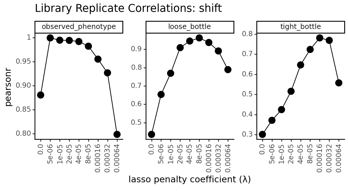
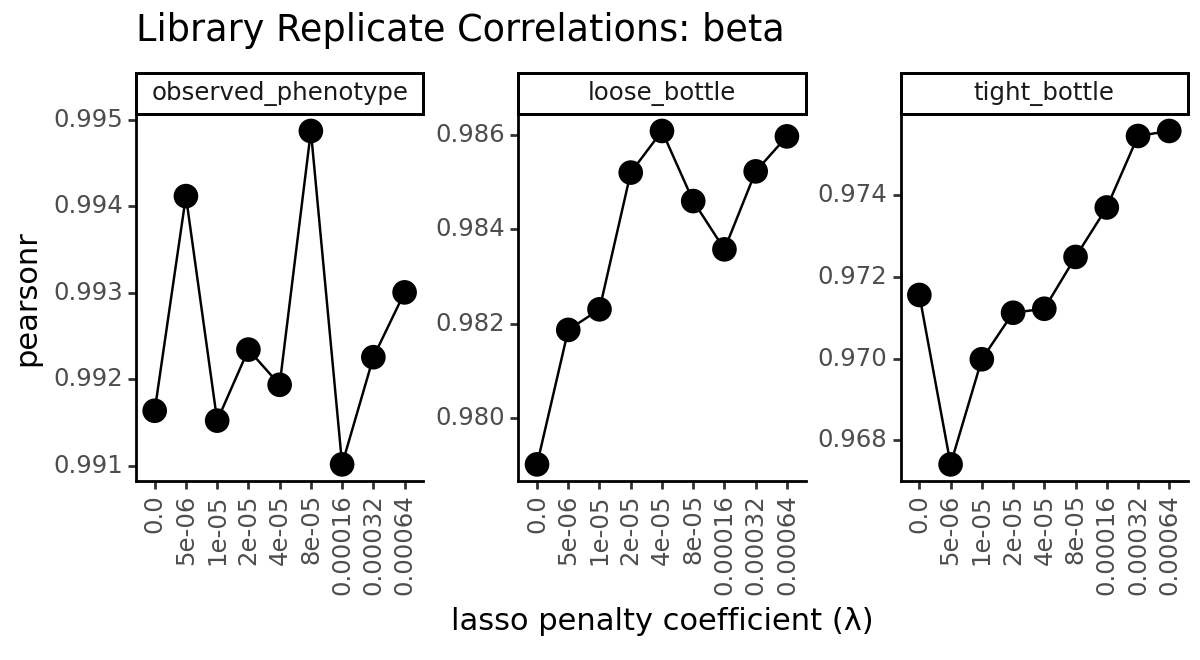
Replicate correlations
Another common metric to look at when evaluating models is to look at the correlation of the inferred mutational effects between the two libraries. We can do this by computing the pearson correlation coefficient between the inferred mutational effects for each mutation in the two libraries using the multidms.ModelCollection.mut_param_dataset_correlation
method.
[49]:
chart, data = model_collection.mut_param_dataset_correlation(return_data=True)
data.head()
[49]:
| datasets | mut_param | correlation | scale_coeff_lasso_shift | |
|---|---|---|---|---|
| 0 | lib_1_loose_bottle_func_score,lib_1_observed_p... | beta | 0.990554 | 0.000000 |
| 0 | lib_1_loose_bottle_func_score,lib_1_observed_p... | beta | 0.992074 | 0.000005 |
| 0 | lib_1_loose_bottle_func_score,lib_1_observed_p... | beta | 0.991360 | 0.000010 |
| 0 | lib_1_loose_bottle_func_score,lib_1_observed_p... | beta | 0.993988 | 0.000020 |
| 0 | lib_1_loose_bottle_func_score,lib_1_observed_p... | beta | 0.994166 | 0.000040 |
By default, the method returns a dataframe giving parameter between each unique pair of datasets, meaning it includes correlations between models fit on different measurement types. We’ll only be comparing models trained the same fitting target combination.
[50]:
data = (
    data
    .assign(
        lib1 = data.datasets.str.split(",").str[0],
        lib2 = data.datasets.str.split(",").str[1],
        measurement_type_1 = lambda x: x["lib1"].str.split("_").str[2:4].str.join("_"),
        measurement_type_2 = lambda x: x["lib2"].str.split("_").str[2:4].str.join("_")
    )
    .query("(measurement_type_1 == measurement_type_2) & (~mut_param.str.contains('predicted_func_score'))")
    .rename(
        {
            "measurement_type_1" : "measurement_type",
        },
        axis=1
    )
    .replace({"shift_h2": "shift"})
    .drop(["lib1", "lib2", "datasets", "measurement_type_2"], axis=1)
)

data.head(10)
[50]:
| mut_param | correlation | scale_coeff_lasso_shift | measurement_type | |
|---|---|---|---|---|
| 0 | beta | 0.979013 | 0.000000 | loose_bottle |
| 0 | beta | 0.981865 | 0.000005 | loose_bottle |
| 0 | beta | 0.982301 | 0.000010 | loose_bottle |
| 0 | beta | 0.985200 | 0.000020 | loose_bottle |
| 0 | beta | 0.986082 | 0.000040 | loose_bottle |
| 0 | beta | 0.984596 | 0.000080 | loose_bottle |
| 0 | beta | 0.983572 | 0.000160 | loose_bottle |
| 0 | beta | 0.985226 | 0.000320 | loose_bottle |
| 0 | beta | 0.985968 | 0.000640 | loose_bottle |
| 0 | shift | 0.435964 | 0.000000 | loose_bottle |
[51]:
data["measurement_type"] = pd.Categorical(
    data["measurement_type"],
    categories=["observed_phenotype", "loose_bottle", "tight_bottle"],
    ordered=True
)
data["mut_param"] = pd.Categorical(
    data["mut_param"],
    categories=["shift", "beta"],
    ordered=True
)

data["scale_coeff_lasso_shift"] = data.scale_coeff_lasso_shift.astype(object)

for parameter, parameter_df in data.groupby("mut_param", observed=True):
    p = (
        ggplot(
            parameter_df
        )
        + geom_line(
            aes(
                x="scale_coeff_lasso_shift",
                y="correlation",
                group="measurement_type"
            ),
        )
        + geom_point(
            aes(
                x="scale_coeff_lasso_shift",
                y="correlation",
            ),
            size=4
        )
        + facet_wrap("measurement_type", scales="free_y")
        + theme_classic()
        + theme(
            figure_size=(6, 3.3),
            axis_text_x=element_text(angle=90),
            panel_grid_major_x=element_blank(),  # no vertical grid lines
        )
        + labs(
            title=f"Library Replicate Correlations: {parameter}",
            x="lasso penalty coefficient (λ)",
            y="pearsonr"
        )
    )
    _ = p.draw(show=True)
[52]:
data.to_csv(f"{csv_output_dir}/library_replicate_correlation.csv", index=False)
data.round(2).head()
[52]:
| mut_param | correlation | scale_coeff_lasso_shift | measurement_type | |
|---|---|---|---|---|
| 0 | beta | 0.98 | 0.0 | loose_bottle |
| 0 | beta | 0.98 | 0.000005 | loose_bottle |
| 0 | beta | 0.98 | 0.00001 | loose_bottle |
| 0 | beta | 0.99 | 0.00002 | loose_bottle |
| 0 | beta | 0.99 | 0.00004 | loose_bottle |
Model vs. truth variant phenotypes
Let’s take a look at how the lasso constraint affects the models’ ability to predict the true latent and observed phenotypes.
First, we grab the model predictions of latent and observed phenotypes for each of the datasets using multidms.Model.get_variants_df.
[53]:
variants_df = pd.concat(
    [
        row.model.get_variants_df(phenotype_as_effect=False)
        .assign(
            library=row.library,
            measurement_type=row.measurement_type,
            scale_coeff_lasso_shift=row.scale_coeff_lasso_shift,
        )
        .rename(
            {
                "predicted_func_score": "predicted_phenotype",
                "predicted_latent": "predicted_latent_phenotype",
                "func_score" : "measured_phenotype",
            },
            axis=1,
        )
        # add enrichments
        .assign(
            predicted_enrichment = lambda x: 2**x['predicted_phenotype'],
            measured_enrichment = lambda x: 2**x['measured_phenotype'],
            fit_idx = idx
        )
        for idx, row in fit_collection_df.iterrows()
    ]
)
variants_df.head()
[53]:
| condition | aa_substitutions | measured_phenotype | var_wrt_ref | predicted_latent_phenotype | predicted_phenotype | library | measurement_type | scale_coeff_lasso_shift | predicted_enrichment | measured_enrichment | fit_idx | |
|---|---|---|---|---|---|---|---|---|---|---|---|---|
| 0 | h1 | V24Q S25R H27P D29L H33C S41L C44F S47F | -5.959752 | V24Q S25R H27P D29L H33C S41L C44F S47F | -10.951781 | -5.962394 | lib_1 | observed_phenotype | 0.0 | 0.016038 | 0.016067 | 0 |
| 1 | h1 | V8P H27T P30* L49P | -5.959753 | V8P H27T P30* L49P | -4.826468 | -5.914732 | lib_1 | observed_phenotype | 0.0 | 0.016576 | 0.016067 | 0 |
| 2 | h1 | V19P V43Q | -5.640393 | V19P V43Q | -2.839960 | -5.630857 | lib_1 | observed_phenotype | 0.0 | 0.020181 | 0.020048 | 0 |
| 3 | h1 | R20Y | 0.005959 | R20Y | 5.107153 | 0.009075 | lib_1 | observed_phenotype | 0.0 | 1.006310 | 1.004139 | 0 |
| 4 | h1 | 0.000000 | 4.938403 | 0.002477 | lib_1 | observed_phenotype | 0.0 | 1.001719 | 1.000000 | 0 |
Next, add the simulated ground truth phenotypes:
[54]:
variants_df  = pd.concat(
    [
        variants_df.query("condition == @homolog")
        .assign(
            true_latent_phenotype = lambda x: x['aa_substitutions'].apply(phenotype_fxn_dict["latentPhenotype"]),
            true_observed_phenotype = lambda x: x['aa_substitutions'].apply(phenotype_fxn_dict["observedPhenotype"]),
            true_enrichment = lambda x: x['aa_substitutions'].apply(phenotype_fxn_dict["observedEnrichment"]),
        )
        for homolog, phenotype_fxn_dict in zip(["h1", "h2"], [phenotype_fxn_dict_h1, phenotype_fxn_dict_h2])
    ]
)

variants_df["measurement_type"] = pd.Categorical(
    variants_df["measurement_type"],
    categories=["observed_phenotype", "loose_bottle", "tight_bottle"],
    ordered=True
)

# As a sanity check let's make sure the true phenotypes match the
# "measured phenotypes" (i.e. fitting targets) for the variants that were trained on ground truth targets
assert np.allclose(
    variants_df.query("measurement_type == 'observed_phenotype'")['measured_phenotype'],
    variants_df.query("measurement_type == 'observed_phenotype'")['true_observed_phenotype'],
)
For clarity, let’s define and arrange the columns we now have:
[55]:
cols = [
    # unique combinations of these make up the model collection that we've fit
    "library", # replicate library,
    "measurement_type", # type of functional score
    "scale_coeff_lasso_shift", # lasso coefficient of model

    # variant defining columns
    "aa_substitutions", # variant substitutions
    "var_wrt_ref", # variant substitutions relative to reference wildtype
    "condition", # homolog

    "measured_phenotype", # the actual target functional score for training, in multidms, this is "func_score"
    "measured_enrichment", # 2 ** measured_func_score

    "predicted_latent_phenotype", # predicted latent phenotype
    "predicted_phenotype", # predicted observed phenotype - or in jesse's case, the "observed phenotype"
    "predicted_enrichment", # predicted enrichment

    "true_latent_phenotype", # true latent phenotype
    "true_observed_phenotype", # true observed phenotype
    "true_enrichment", # true enrichment
]
# variants_df[cols].round(2).head()
Add correlation of ground truth targets / predicted phenotypes to the fit collection dataframe and plot them:
[56]:
for idx, model_variants_df in variants_df.groupby("fit_idx"):
    for metric_fxn, metric_name in zip([series_corr, series_mae], ["corr", "mae"]):
        fit_collection_df.loc[idx, f"variant_phenotype_{metric_name}"] = metric_fxn(
            model_variants_df["measured_phenotype"],
            model_variants_df["predicted_phenotype"]
        )

fit_collection_df[["scale_coeff_lasso_shift", "dataset_name", "variant_phenotype_corr", "variant_phenotype_mae"]].head()
[56]:
| scale_coeff_lasso_shift | dataset_name | variant_phenotype_corr | variant_phenotype_mae | |
|---|---|---|---|---|
| 0 | 0.0 | lib_1_observed_phenotype_func_score | 0.999985 | 8.611429e-06 |
| 1 | 0.000005 | lib_1_observed_phenotype_func_score | 0.999994 | 5.973305e-07 |
| 2 | 0.00001 | lib_1_observed_phenotype_func_score | 0.999989 | 1.648540e-04 |
| 3 | 0.00002 | lib_1_observed_phenotype_func_score | 0.999980 | 1.652058e-04 |
| 4 | 0.00004 | lib_1_observed_phenotype_func_score | 0.999950 | 3.538619e-06 |
[57]:
# for metric in ["corr", "mae"]:
data = fit_collection_df[["library", "measurement_type", "scale_coeff_lasso_shift", "dataset_name", "variant_phenotype_corr", "variant_phenotype_mae"]]
metric = "corr"
p = (
    ggplot(
        data
        .assign(
            measurement_library = lambda x: x["library"] + "_" + x["measurement_type"].astype(str)
        )
    )
    + geom_line(
        aes(
            x="scale_coeff_lasso_shift",
            y=f"variant_phenotype_{metric}",
            group="measurement_library",
        ),
    )
    + geom_point(
        aes(
            x="scale_coeff_lasso_shift",
            y=f"variant_phenotype_{metric}",
            shape="library"
        ),
        size=4
    )
    + facet_wrap("measurement_type", scales="free_y")
    + theme_classic()
    + theme(
        figure_size=(6.5, 3.3),
        axis_text_x=element_text(angle=90),
        panel_grid_major_x=element_blank(),  # no vertical grid lines
    )
    + labs(
        title=f"Predicted Vs. True Variant Phenotype",
        x="lasso penalty coefficient ($\lambda_{L1}$)",
        y="pearsonr" if metric == "corr" else "mean absolute error"
    )
)
_ = p.draw(show=True)
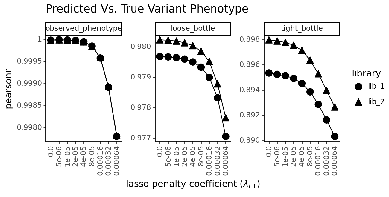
As expected, the lasso constraint has a negative effect on the models’ ability to predict the true latent and observed phenotypes. This is because a model with more freedom to choose parameters is likely to overfit to the training data.
[58]:
data.to_csv(f"{csv_output_dir}/model_vs_truth_variant_phenotype.csv", index=False)
data.round(2).head()
[58]:
| library | measurement_type | scale_coeff_lasso_shift | dataset_name | variant_phenotype_corr | variant_phenotype_mae | |
|---|---|---|---|---|---|---|
| 0 | lib_1 | observed_phenotype | 0.0 | lib_1_observed_phenotype_func_score | 1.0 | 0.0 |
| 1 | lib_1 | observed_phenotype | 0.000005 | lib_1_observed_phenotype_func_score | 1.0 | 0.0 |
| 2 | lib_1 | observed_phenotype | 0.00001 | lib_1_observed_phenotype_func_score | 1.0 | 0.0 |
| 3 | lib_1 | observed_phenotype | 0.00002 | lib_1_observed_phenotype_func_score | 1.0 | 0.0 |
| 4 | lib_1 | observed_phenotype | 0.00004 | lib_1_observed_phenotype_func_score | 1.0 | 0.0 |
Cross validation
Above, we saw evidence that the lasso negatively impacts the model performance on the training data. To test for overfitting, we can perform cross validation to test that the model is actually more accurate on unseen data.
[59]:
train, test = [], {}
for (library, measurement), fs_df in func_scores.rename(columns={"homolog":"condition"}).groupby(["library", "func_score_type"]):

    if "enrichment" in measurement:
        continue

    dataset = fs_df.sample(frac=1, random_state=seed)
    train_split, test_split = dataset.iloc[:int(len(dataset) * train_frac)], dataset.iloc[int(len(dataset) * train_frac):]
    name = f"{library}_{measurement}"

    train.append(
        multidms.Data(
            train_split,
            reference="h1",
            alphabet = multidms.AAS_WITHSTOP_WITHGAP,
            verbose=False,
            name = name
        )
    )

    test[name] = test_split
[60]:
fitting_params["dataset"] = train
_, _, fit_collection_cv = multidms.model_collection.fit_models(fitting_params)
The multidms.ModelCollection.add_validation_loss method takes in unseen data, computes model loss on that data, and appends it to the ModelCollection.fit_models dataframe.
[ ]:
mc = multidms.model_collection.ModelCollection(fit_collection_cv)
mc.add_validation_loss(test, overwrite=True)
[62]:
mc.fit_models[[c for c in mc.fit_models.columns if "loss" in c]].head()
[62]:
| step_loss | h1_loss_training | h2_loss_training | total_loss_training | h1_loss_validation | h2_loss_validation | total_loss_validation | |
|---|---|---|---|---|---|---|---|
| 0 | [6.3576507568359375, 0.00012060716835549101] | 0.000078 | 0.000043 | 0.000121 | 0.001116 | 0.000479 | 0.001595 |
| 1 | [6.3576507568359375, 8.627029455965385e-05] | 0.000032 | 0.000054 | 0.000086 | 0.000089 | 0.000804 | 0.000893 |
| 2 | [6.3576507568359375, 0.00013628264423459768] | 0.000053 | 0.000083 | 0.000136 | 0.000207 | 0.001059 | 0.001266 |
| 3 | [6.3576507568359375, 0.000258071580901742] | 0.000117 | 0.000141 | 0.000258 | 0.000618 | 0.001297 | 0.001914 |
| 4 | [6.3576507568359375, 0.0006348328315652907] | 0.000305 | 0.000330 | 0.000635 | 0.001270 | 0.001042 | 0.002312 |
[63]:
data = mc.fit_models

data["library"] = data["dataset_name"].str.split("_").str[0:2].str.join("_")
data["measurement_type"] = data["dataset_name"].str.split("_").str[2:4].str.join("_")
data["measurement_type"] = pd.Categorical(
    data["measurement_type"],
    categories=["observed_phenotype", "loose_bottle", "tight_bottle"],
    ordered=True
)

data = (
    data
    .melt(
        id_vars=["scale_coeff_lasso_shift", "library", "measurement_type"],
        value_vars=["total_loss_training", "total_loss_validation"],
        var_name="dataset",
        value_name="loss",
    )
    .assign(
        dataset = lambda x: x["dataset"].str.replace("_loss", "")
    )
    .assign(
        lib_dataset = lambda x: x["library"] + " " + x["dataset"]
    )
)
p = (
    ggplot(data)
    + geom_line(
        aes(
            x="scale_coeff_lasso_shift",
            y=f"loss",
            group="lib_dataset",
        )
    )
    + geom_point(
        aes(
            x="scale_coeff_lasso_shift",
            y=f"loss",
            fill="dataset",
            shape="library"
        ),
        size=4
    )
    + facet_wrap("measurement_type", scales="free_y")
    + theme_classic()
    + theme(
        figure_size=(6.5, 3.3),
        axis_text_x=element_text(angle=90),
        panel_grid_major_x=element_blank(),  # no vertical grid lines
    )
    + labs(
        x="lasso penalty coefficient (λ)",
        y="Huber loss w/o penalty"
    )
)
_ = p.draw(show=True)
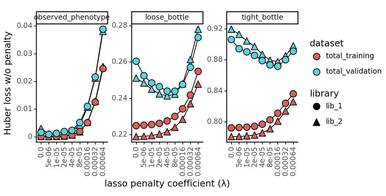
Above we can see that indeed for both the loose and tight bottleneck datasets, the lasso constraint provides a more robust model to unseen data. We don’t however see this effect for the models trained on ground truth observed phenotypes, as there is no noise for the models to overfit to.
[64]:
data.to_csv(f"{csv_output_dir}/cross_validation_loss.csv", index=False)
data.round(2).head()
[64]:
| scale_coeff_lasso_shift | library | measurement_type | dataset | loss | lib_dataset | |
|---|---|---|---|---|---|---|
| 0 | 0.0 | lib_1 | observed_phenotype | total_training | 0.0 | lib_1 total_training |
| 1 | 0.000005 | lib_1 | observed_phenotype | total_training | 0.0 | lib_1 total_training |
| 2 | 0.00001 | lib_1 | observed_phenotype | total_training | 0.0 | lib_1 total_training |
| 3 | 0.00002 | lib_1 | observed_phenotype | total_training | 0.0 | lib_1 total_training |
| 4 | 0.00004 | lib_1 | observed_phenotype | total_training | 0.0 | lib_1 total_training |
Final Selection
This analysis above provides a number of clues to inform our choice of model. With empricial data we obviously won’t have comparisons to the ground truth values, and thus the choice of a lasso penalty will laregely depend on the shift parameter sparsity, correlation of inferred mutational effects between replicate libraries, and cross validation performance. Focusing on the loose bottleneck training dataset (a fairly realistic level of noise that we often observe in real experiments), it seems that a lasso penalty of \(1e-4\) provides a false positive rate of nearly zero (i.e. the stop codon sparsity \(\approx 100\%\)), a good correlation of inferred mutational effects between replicate libraries (>0.95 pearsonr), and a relatively low loss on validation when compared to the other models.
To validate the ability to correctly infer the shape of epistasis, we’ll plot the inferred global epistasis function for each of the models, and compare it to the true global epistasis function.
[65]:
data = variants_df.query(f"scale_coeff_lasso_shift == {lasso_choice}")
for x, y in itertools.combinations(
    ["predicted_latent_phenotype", "predicted_phenotype", "measured_phenotype"], 2
):
    p = (
        ggplot(data.sample(frac=1.0))
        + geom_point(
            aes(
                x=x,
                y=y
            ),
            alpha=0.05,
            color="grey"
        )
        + ylab(y)
        + xlab(x)
        + facet_grid("~measurement_type")
        + theme_classic()
        + theme(
            figure_size=(6.5, 3.5),
            axis_text_x=element_text(angle=90),
        )
    )

    if x == "predicted_latent_phenotype":
        p+= geom_point(
            aes(
                x="true_latent_phenotype",
                y="true_observed_phenotype"
            ),
            size=0.5,
        )
    else:
        p += geom_abline(
            slope=1,
            intercept=0,
        )

    _ = p.draw(show=True)
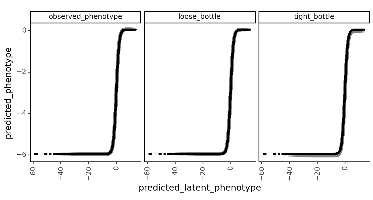
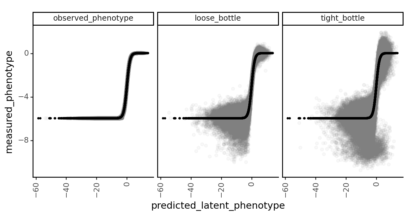
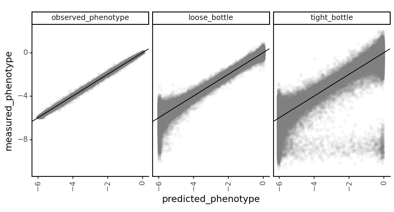
Plot model vs. measured (functional score) vs. ground truth enrichments.
[66]:
p = (
    ggplot(
        data.melt(
            # id_vars=["measurement_type", "library", "condition", "true_enrichment"],
            id_vars=["measurement_type", "library", "true_enrichment"],
            value_vars=["predicted_enrichment", "measured_enrichment"],
            var_name="enrichment_type",
            value_name="enrichment",
        ),
        # variants_df,
        aes("true_enrichment", "enrichment"),
    )
    + geom_abline(
        slope=1,
        intercept=0,
        # alpha=0.5,
        # size=0.5,
    )
    + geom_point(alpha=0.05, size=0.5)
    + facet_grid("enrichment_type~measurement_type", scales="free_y")
    + theme_classic()
    + theme(
        figure_size=(6.5, 5),
    )
)

_ = p.draw(show=True)
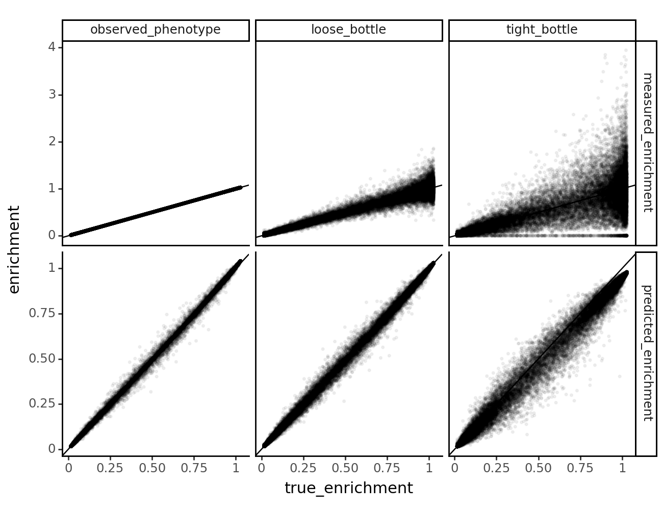
Amazingly, the model does better at predicting true enrichments than even the counts based functional scores!
Finally, let’s plot the relationship between the model’s inferred shifts, and the ground truth shifts.
[67]:
# plot correlations of true and predicted shifts
collection_muts_df["measurement_type"] = pd.Categorical(
    collection_muts_df["measurement_type"],
    categories=["observed_phenotype", "loose_bottle", "tight_bottle"],
    ordered=True
)

for (x, y) in itertools.combinations(
    ["true_shift", "predicted_shift_h2"], 2
):
    p = (
        ggplot(collection_muts_df.query(f"scale_coeff_lasso_shift == {lasso_choice}"))
        + geom_point(
            aes(
                x=x,
                y=y
            ),
            alpha=0.5,
        )
        + geom_abline(
            slope=1,
            intercept=0,
        )
        + ylab(y)
        + xlab(x)
        + facet_grid("library~measurement_type")
        + theme_classic()
        + theme(
            figure_size=(6.5, 5),
            axis_text_x=element_text(angle=90),
        )
    )
    _ = p.draw(show=True)